University of Southampton Falmouth Field Course 2013 26th June -
28th June 2013 -
Falmouth Tides (UTC): LW 0300 0.4m
HW 0846 4.8m
LW 1518 0.6m
HW 2101 5.0m
Cloud cover: 100%
Sea State: Flat -
Location: 50° 12.57’N 005° 01.37’W
Introduction
On the afternoon of the 28th June 2013, measurements were taken at King Harry Pontoon to create a time series of oceanographic data. Data was collected at every 30 minutes from 12:45 UTC through to 15:45 UTC from the western side of the pontoon. As these results only resemble half a day, we extrapolated data taken by Group 13 in the morning. By expanding the data a time series representative of the full day and therefore the entire period of the ebb tide can be shown. The data from the pontoon is used to observe the physical and chemical changes in the water over the tidal cycle with time. Measurements for: temperature; salinity; pH; dissolved oxygen were taken using a YSI multiprobe. Current velocity and direction, and light intensity were also measured.
Methods
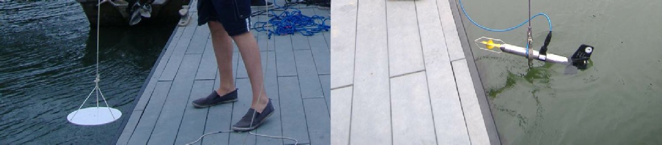
Secchi disk depth and light attenuation measurement
To determine the depth, the Secchi disk was lowered over the side until it hit the bottom and the rope went slack. This depth was measured using the knots in the rope every metre. This was an approximate depth that was used as a maximum to prevent damage to the other, more delicate, instruments.
To obtain the light attenuation, the Secchi disk was slowly lowered over the side until the white top of the disk was no longer visible. This depth was noted down and used to calculate the approximate light attenuation k (k=1.44/z; where z=Secchi depth (m)). The Secchi depth was multiplied by 3 to calculate the euphotic depth.
Light Meter
An initial calibration was taken with both sensors next to one another before each
set of measurements were taken. The water sensor (LI-
Current Meter
The tow fish was lowered into the water just below the surface of the water column to measure both current velocity and direction. The tow fish was then lowered to a depth of one metre where the measurements were repeated, and compared to the surface.
YSI Probe
The probe was lowered to the surface where temperature (°C), salinity (PSU), pH, DO2 (%), DO (mg/L) and depth (m) were recorded. A second set of measurements of these parameters were taken from at the bottom depth.
Results
Light attenuation coefficient
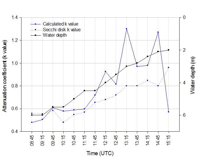
The attenuation coefficient (k value), calculated from the light meter data, was observed to increase as the water column depth decreased. This is shown in figure T.1, where the k value increased from 0.47 at 08:45 UTC to 1.27 at 14:45, whereas the depth decreased from 6m to 2.1m. The k value calculated at 15:15 UTC is believed to be an anomaly. The k values that were calculated from the secchi disk depth were also seen to follow a similar trend, increasing as the water column got shallower.
Figure T.1: The calculated k value and the secchi disk k value across the time series. The depth is also shown in black. (Click to enlarge)
Salinity
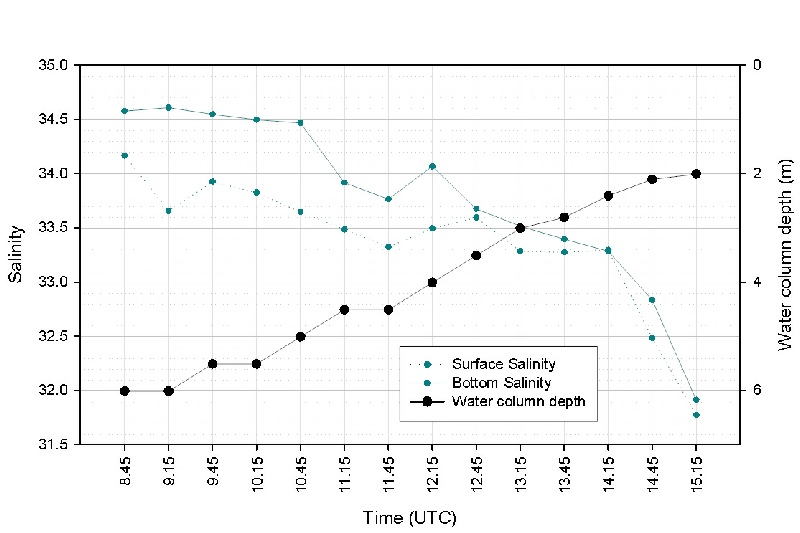
As the water column depth decreased, it was also observed that the salinity decreased.
The initial values at the start of the time series are similar to those found in
the western English Channel, approximately 34-
Figure T.2: The change in salinity at the surface and at the bottom (blue) and the change in water column depth (black) over the time series. (Click to enlarge)
Dissolved Oxygen
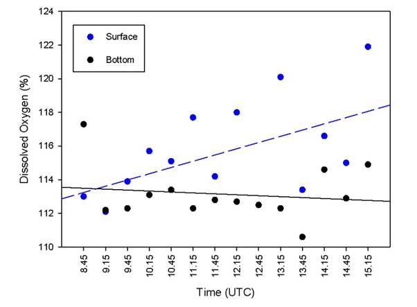
The dissolved oxygen at the surface of the river can be seen to increase across the time series (figure T.3). At 8:45 UTC the DO can be seen to be 113%, where the water depth was deepest. This value increased to 118% at 15:15 UTC with a shallower water column depth. The bottom DO was observed to remain constant throughout the day at approximately 113%.
Figure T.3: The change in dissolved oxygen for the surface (dashed) and bottom (dotted) across the time series with linear regression. (Click to enlarge)
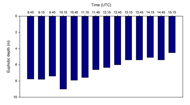
Euphotic Zone
From multiplying the Secchi disk depth by 3, the euphotic zone depth was obtained. This slightly decreased across the time series from 7.75m at 8:45 UTC to 4.5m at 15:15 UTC. This indicates that the euphotic zone depth was consistently greater than the water column depth.
Figure T.4: The change in approximate euphotic depth across the time series. (Click to enlarge)
Temperature
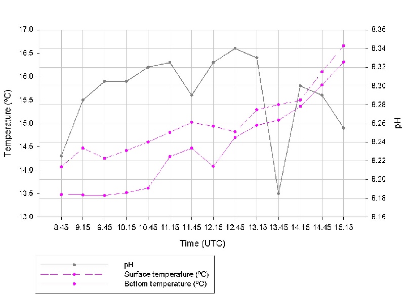
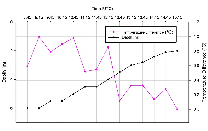
When the depth of the water column decreased with the ebb tide, it was observed that both the temperature of the surface and the temperature of the bottom water increased (figure T.5). The surface water temperature was also constantly warmer than the deeper water. When comparing the difference between the surface temperature and the bottom temperature, it was observed that the temperature difference decreased as the depth of the water column became shallower (figure T.6).
Figure T.5: The change in temperature of the surface and bottom (pink) and the average change in pH (grey) over the time series. (Click to enlarge)
Figure T.6: The time series of the difference between surface and bottom temperatures (pink) and the decrease of the depth of the water column (black). (Click to enlarge)
pH
The pH was shown to initially increase from 08:45 UTC (figure T.5). This appeared to plateau to 8.32pH at 11:45 UTC before decreasing in the afternoon. The measurement taken at 13:45 UTC is believed to be an anomaly.
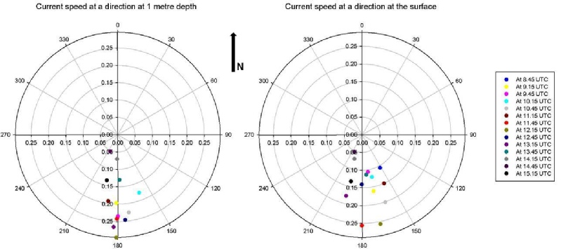
Current Speed and Direction
In the polar plot for current direction; 0° represents an upstream flow in the North direction, and 180° represents a downstream flow out of the estuary (Figure T.7). The graphs both show that there was a continuous flow out of the estuary. They also show that the surface speed was, on average, lower than at a depth of 1 metre. The current velocities were observed to become slower as time went on as the end of the ebb tide approached.
Figure T.7: The current speed and direction at the surface (Left image) and at 1 metre depth (right image)at each time of the time series. (Click to enlarge)
Conclusions
Light Attenuation (figure T.1)
The graph tells us that the light beam in the water is weakened as time passed, which
relates to the decreasing depth as the tide was ebbing. The ebbing tide causes disturbance
on the seabed and particles become suspended. Also, the river water coming from upstream
may have had a higher concentration of suspended particles present. The data point
for the calculated k value at 15:15 UTC is believed to be an anomaly. Every 15 minutes
the King Harry Ferry crossed the river from Foeck to Roseland which created a large
wake that could lead to increased mixing of the water column and re-
Salinity (figure T.2)
When comparing the salinity changes over the time, it was observed that the salinity
decreased with the ebb tide. The initial salinity was between 34-
Dissolved Oxygen (figure T.3)
The dissolved oxygen (DO) increased steadily in the surface water over the time series. This increase in dissolved O2 can be related to the increase in light intensity throughout the day. As the light intensity increases; photosynthetic activity in the water also increases. This increases O2 production releasing a greater amount of O2 into the water. In the bottom water, the DO was observed to remain constant. The euphotic zone is deeper than the water column, suggesting that there would still be primary producers present, and any removal of oxygen is from the presence of aerobic organisms present in the benthic habitat.
Euphotic Zone (figure T.4)
Light levels were inconsistent due to fluctuation in cloud coverage over the sampling period. As can be seen in Figure T.4, the euphotic zone depth vertically rose with the outgoing tide throughout the afternoon. This is to be expected as the river water contains a higher concentration of particulate matter; this recession of higher salinity water can be seen as the salinity drops throughout the afternoon and the water depth decreases. The euphotic depth was greater than the water depth throughout the time series which means there is always light reaching the seabed. This makes it possible for multiple biological communities to develop.
Temperatures (figure T.5 and T.6)
When the depth of the water column decreased with the ebb tide, it was observed that both the temperature of the surface and the temperature of the bottom water increased (figure T.5). This is due to the increase in air temperature throughout the day, warming the water column from the surface, downwards. The surface waters have a greater temperature than the bottom and the difference between these two temperatures decreased with the ebb tide (figure T.6). This is due to an increase in mixing as the water column becomes shallower.
pH (figure T.5)
pH was not expected to change much, however, due to the logarithmic nature of the scale with which we measure pH, any small changes can resemble large changes in ion concentration in the water. Changes remain minimal as a result of the bicarbonate buffering characteristic of seawater. The value measured at 13:45 UTC is believed to be an anomaly, potentially from a pollutant from upstream.
Current Speed and Direction (figure T.7)
The graphs both show that there was a continuous flow out of the estuary. This is unsurprising as we know that the tide was due to be ebbing during the time of sampling. They also show that the surface speed was lower, on average, than at a depth of 1 metre. This suggests that tide flow was dominant and wind shear was minimal. The current velocities were observed to become slower as time went on as the ebb tide ended.
References
Groom, S., Martinez-
Fal River Time Series
| Introduction |
| Methods |
| Results |
| Discussion |
| Physical |
| Chemical |
| Biological |
| Physical |
| Chemical |
| Biological |
| Introduction |
| Methods |
| Results |
| Discussion |
| Physical |
| Chemical |
| Biology |
| Physical |
| Chemical |
| Biology |