Home Offshore Time Series Geophysical Estuary

University of Southampton Falmouth Field Course 2013    26th June - 6th July 2013    Group 9

26th June 2013 - Offshore Sampling
Falmouth Tides (UTC): HW 07:20 5.1m
LW 13:50 0.3m
Cloud cover: 100% - 0%
Sea State: Flat - Slight
Air Temperature: 14.9°C

Physical Discussion

Stratification Index (S)

A stratification index (S) equal to or higher than 3 represents highly stratified waters, an S value of –2 indicates highly turbulent waters and an S value equal to 1.5 represents a transition zone, thus providing optimum conditions for primary production (Simpson and Sharples, 2012). The S values for all stations (figure OP.1) are close to or higher than 3, which is indicative of stratified conditions within the vicinity of sampling stations. Overall, stratification index values (SI) at all stations show a well stratified water column within the sample area, where S values range between 3.923 (Station 1) and 2.757 (Station 2).

Temperature

The general trend for all stations is a decrease in temperature with depth (figure OP.2). Mixing and the low temperature of the water column at Station 4 would be due to the effect of surface wind mixing as well as tidal mixing, the influence of which increases as the water depth decreases. The development of the observed seasonal thermocline in the study area is typical of the coastal waters of south-west England (Smyth et al., 2010). The thermocline at 30 metres depth is temperature driven as temperature variations (4°C) (figure OP.2) are much larger than variations in salinity (0.16) (figure OP.3). The water column at Station 2 also displays stratification, however it is less pronounced than at Station 1. The depth of the thermocline decreases towards the mouth of the estuary, i.e. towards Station 4, due to the decrease in water depth, where the effects of tidal and wind mixing are most pronounced. The thermocline between Station 1 and Station 2 shallows with depth by approximately 20 metres, which can be expected as the average water depth between stations decreases.

Salinity

Small range in salinity of 0.17 units between all four stations (figure OP.10) is to be exected, as station locations are offshore from Falmouth and thus the influnce of fresh water input from rivers discharging into Fal and Helford estuaries is not detected. The observed spike in the salinity profile at Station 2 at approximately 20 m depth (figure OP.8) is attributed to the mismaches in CTD sensors response time (mainly conductivity cell and temperature transmissometer). This corresponds to a spike at approximately 20 m seen in the density profile (figure OP.4), which is to be expected, as density is derived from salinity, temperature and pressure. The greater the salinity spike, the greater the lag in response time between the two sensors.

Figure OP.8: CTD derived vertical profiles of salinity at all stations showing salinity ‘spike’ at 20 m depth

Density

The depth of the pycnocline decreases from Station 1 to Station 2 and progressively disappears towards Station 3 and completely disappears at Station 4 (figure OP.4), where the effect of tidal and wind induced mixing increase and are more pronounced as the water depth decreases towards the mouth of the estuary. The developed pycnoclines at Stations 1 and 2 represent staticaly stable water columns, while waters at Stations 3 and 4 exibit turbulent character. This is in correspondence with the occurrence and change in flood and ebb tide flows (HW at 07:20 (UTC) and LW at 13:50 (UTC)).

Richardson Number (Ri)

Richardson number (Ri) is given by: Ri = N2/(du/dz)2, where N = Brunt-Vaisala frequency (N = (g/ρ)*(dρ/dz) - g2/c2) and du/dz = velocity gradient, i.e. shear.

For shallow estuarine and offshore environments the following simplifications could be applied: pressure effect can be neglected, as well as g2/c2 term (g (m s-1) gravitational constant and c, speed of sound in water (taken as 1500 m s-1)). As stratification plays a significant part, the main stabilising buoyancy (dρ/dz) is between the density difference of upper and lower layers within the water column. Here, the above mentioned simplification has been adopted and Ri numbers have been calculated for all stations at 1 m intervals. The following formula was used: Ri = [g*(ρ2-ρ1)*h]/ (ρ*u2), where, g = 9.810 ms-2 , ρ1 (kg m-3) and ρ2 (kg m-3) = mean densities of respective layers, h = 1 m, ρ = 1025 kg m-3, used at all stations as mean density of water and u (m s-1) = mean velocity of the corresponding water layer within the water column at a particular station.

Current velocity values for each station have been taken from the ADCP discharge summary table.

Figure OP.9: Vertical profiles of Richardson numbers at all stations

Overall, calculated Ri numbers at all stations (figure OP.9) fall below 0.25, indicating that the flow at all four stations exhibits turbulent behaviour. It could be said that that the Ri values in figure OP.9 do not correspond to the stratification index values, which suggests that the water column between the stations is highly stratified. 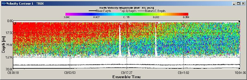However, flows are never truly laminar (Pickard and Emery, 1990), which can be seen from the current velocity (m s-1) contour profiles for all four stations (figures OP.10, OP.11, OP.12 & OP.13). The highest current velocity (0.441 m s-1) was observed at Station 2, corresponding to the lowest stratification index (2.757), while the lowest current velocity (0.197 m s-1) was observed at Station 1, which corresponds to the highest stratification index (3.923). Therefore, there is an inverse relationship between the two parameters, and consequently, Richardson number is inversely proportional to the current velocity, which is supported by highest Ri values of 0.12 at Station 1 (figure OP.8) and lowest current velocity (0.197 m s-1). Variations of Ri values between stations are due to the variations in current velocity with depth, caused by the frictional stresses arising from bottom friction and friction between layers (Simpson and Sharples 2012). Variability of current velocity between stations is evident from backscatter contour plots (figures OP.10, OP.11, OP.12 & OP.13). Although ADCP transect velocity contour plots do not show velocities at the bottom of the water column (no ADCP data available for bottom cells), current velocities at each stations would be minimal at or near the surface due to shear, induced at the sea bed and water column interface.  

Figure OP.10 ADCP derived current velocity contour plot between Black Rock and Station 1

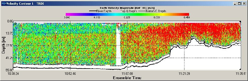
Figure OP.11 ADCP derived current velocity contour plot between Station 1 and Station 2

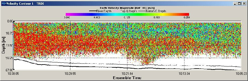
Figure OP.12 ADCP derived current velocity contour plot between Station 2 and Station 3

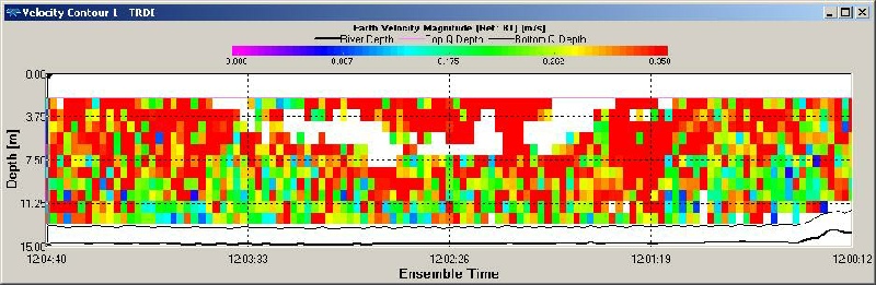
Figure OP.13 ADCP derived current velocity contour plot between Station 3 and Station 4

Fluorescence

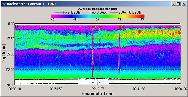
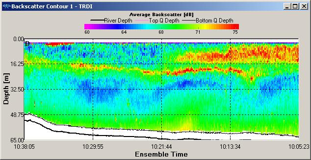
Backscatter contour plots for Station 1 and Station 2 (figure OP.14 & OP.15) show the presence of zooplankton species between subsurface depths of 6m and 27.60m for Station 1 and subsurface depths of 6m and 22.50m for Station 2, which indicates the presence of zooankton. This corresponds to fluorescence peaks at ~ 30 m depth at Station 1 (0.25 µg/ L) and at ~ 17 m at Station 2 (0.21 µg/ L), indicating that the bottom of the euphotic zone (figure OP.6) provides optimum growth conditions for zooplankton species at Station 1 and Station 2. Increased backscatter in both contour plots (figure OP.14 & OP.15) is due to re-suspension of sediment in the water column from tidal current interference with the sea bed.  

Figure OP.14 ADCP derived backscatter plot between Black Rock and Station 1

Figure OP.15 ADCP derived backscatter plot between Station 1 and Station 2

Transmission

Transmission measures the percentage of light penetration through the water column and is used as a proxy for the amount of suspended particulate matter (SPM) (Towns, 2010). At Stations 1 and 2 the profiles show highly variable transmission through the water column (figure OP.7), due to stratified conditions (figure OP.2 & OP.4). At Station 1 the sharp decrease in transmission at approximately 30m depth is most likely due to a peak in phytoplankton numbers, which creates scattering within the path-length of the transmissometer. This correlates to the spike in fluorescence seen at the same depth in Station 1 (figure OP.6). A similar trend can be seen at Station 2 at approximately 17m depth. Stations 3 and 4 show little variablilty as the water columns are well mixed, suggesting SPM is more evenly distributed throughout the water column.

Linking physical conditions with phytoplankton abundance and distribution within the water column

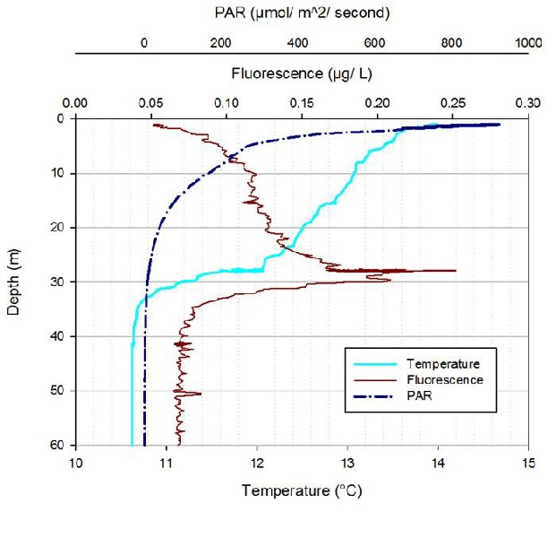
Figure OP.16: CTD derived vertical profiles of PAR, fluorescence and Temperature  at Station 1

Combined vertical profiles of temperature, fluorescence and photosynthetic active radiation (PAR) clearly show the effect of light availability and temperature on phytoplankton species abundance (fluorescence vertical profile) and distribution within the water column. Fluorescence is a measure of chlorophyll a (Chl a) concentrations (µg/ L) and the observed peak at approximately 27.50m depth corresponds to the Chl a maximum depth, which is supported by highest phytoplankton count of 3100 cellsL-1 (Chaetoceros spp.) collected at 27m. In relation to the fluorescence peak between 25m and 30m, mixing at the thermocline can bring nutrient-rich water from below the thermocline up into the euphotic zone, and as nutrient and light availability and temperature are the main controlling factors for primary production (Kirk, 2011), this provides optimum conditions for phytoplankton growth.

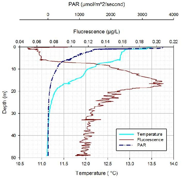
Figure OP.17: CTD derived vertical profiles of PAR, fluorescence and temperature at Station 2

Station 2 combined vertical profiles of temperature, fluorescence and PAR show the same trend seen at Station 1 (figure OP.16), however, the thermocline is shallower (between 15 and 20m). This results in the fluorescence peak occurring at this depth range as well. However, the maximum count number of phytoplankton cells is 26000 cellsL-1 (Chaetoceros spp), recorded at 32.5m depth, which does not correlate to the predicted depth range of optimum conditions. This could be due to localised entrapment of upper water layers and the presence of diatoms below the thermocline can be expected as they are more suited to mixed water environment. Diatoms also migrate to regions of higher nutrient concentrations for nutrient uptake by endocytosis for metabolic processes before returning above the photic zone for photosynthesis.

References

Dyer, K., 1983, Mixing caused by lateral internal seiching within a partially mixed estuary, Estuarine and Coastal Shelf Science, Issue 26, pp. 51 – 66

Kirk, J., 2011, Light and Photosynthesis in Aquatic Ecosystems, Chapter 6.3: Downward irradiance-PAR, Cambridge University Press, Cambridge, UK

Pickard and Emery, 1990, Descriptive Physical Oceanography, Chippenham, Wiltshire, UK

Simpson, J.  and Sharples, J. 2012, Introduction to the Physical and Biological Oceanography of Shelf Seas, , Cambridge University Press, Cambridge, UK

Smyth, T., Fishwick, J., Al-Moosawi, L., Cummings, D., Harris, C., Kitidis, V., Rees, A., Martinez - Vicente, V., and Woodward, E., 2010, A broad spatio – temporal view of the Western English Channel Observatory, Journal of Plankton Research, Vol. 32, pp. 585 - 601

Towns, J. 2010, Relationship of light transmission, stratification and fluorescence in the hypoxic region of Texas-Louisiana Shelf in Spring/Summer 2009, Undergraduate Research Scholar Thesis, Texas A&M University

Viljanen, M. Holopainen, A-L. Bilvenuoinen, R. 1999, Fluorometer measurements and transmission of light in different parts of Lake Ladoga, Boreal Environment Research, Vol 4, pp239-244

Offshore