University of Southampton Falmouth Field Course 2013 26th June -
4th July 2013 – Estuary Sampling
Falmouth Tides (UTC): HW 02:09 4.20m
LW 09:31 1.50m
HW 15:39 4.30m
LW 22.03 1.5m
Chemical Discussion
Depth Profiles
Chlorophyll is an indicator of phytoplankton biomass and therefore is a useful measurement to be taken through the water column to monitor biological activity (Boyer et al. 2009). Figure EC.1 shows that the chlorophyll at each depth decreases at stations 4,5 and 6. Unfortunately due to storage and time restrictions it was not possible to sample phytoplankton throughout the water column, but only at the surface. This was the same with dissolved oxygen, though at stations 1, 8 and 7 it was possible to take more than one dissolved oxygen sample providing us with a partial vertical profile. Since there is no phytoplankton biomass vertical profile it is not possible to say with certainty the decrease in chlorophyll with depth is directly related to a decrease in phytoplankton population as we do not know what the phytoplankton population was at depth.
Figure EC.2 shows the dissolved oxygen saturation percentage at each station at different depths. At station one the oxygen percentage decreases within the first 5m but the chlorophyll increases. This is unexpected as it would be predicted as chlorophyll concentration increases, the phytoplankton biomass increases proportionally so the dissolved oxygen concentration in the water should increase. This is because phytoplankton are photosynthetic organisms and therefore take up carbon dioxide and release oxygen, consequently increasing the dissolved oxygen percentage in the water (McAllister et al. 1964) A possible explanation for this unusual result could be the shallowness of the estuary keeping plankton in the subsurface area as the water column is so shallow. Oxygen content is higher in the subsurface sample indicating phytoplankton is high here but phytoplankton biomass decreases with depth.
Figure EC.5 shows the dissolved silicon vertical profiles at each station. It shows at station one dissolved silicon levels are highest in the subsurface sample indicating diatom presence. Diatoms use silicon in their frustules and therefore deplete silicon levels in the water (Yool et al. 2002). Figure EB.2 shows at station one Thalassiosira eccentric, a diatom species (Hallegraff 1984), was counted in the samples. This explains the higher silicon content in the subsurface sample. Figure EC.3 shows that the nitrate level in the subsurface sample at station one is not depleted. This implies that this area is not nitrate limited as nitrate is requited by phytoplankton for growth. Phosphate is also not depleted in the subsurface sample, showing that the phosphate is not limiting phytoplankton growth either.
Station 4 and 5 are shown in figure EC.1 as having decreasing chlorophyll levels with increasing depth. This means there is decreasing phytoplankton biomass with depth. This will be because of decreasing light levels as more wavelengths are absorbed with deeper depths. Phytoplankton are primary producers and therefore photosynthesise and so their biomass decrease with decreasing light levels as they cannot survive at low intensities. Figure EB.2 shows both diatoms and dinoflagellates were present at station 4 and this explains the depleted dissolved silicon levels. Phytoplankton counts for station 5 were not conducted and the silicon level increases with depth. This suggests there is cooler (figure EP.1), more saline water underneath the fresher water (figure EP.2) bringing nutrients from the ocean into the estuary therefore increasing silicon levels with depth (figure EC.5). Both phosphate and nitrate levels are not depleted in the subsurface levels implying this area is also not nutrient limited. Another parameter is limiting the growth in this region, for example iron (Kolber et al. 1994). Silicon levels are not depleted either and dissolved oxygen levels are not extremely suggesting phytoplankton blooms are not present here.
Stations 6 and 7 have very different vertical profile to stations 1, 4 and 5. These stations have deeper depths than previous stations and have a chlorophyll blooms at approximately 6m depth (figure EC.1). Many diatoms and some dinoflagellates were counted at station 6, but no counts were taken at station 7. If phytoplankton had been counted at station 7 similar species would have been found. Figure EC.2 shows the oxygen concentration at this chlorophyll bloom is considerably higher than at previous stations. This supports the evidence that a phytoplankton bloom was observed at a depth of approximately 6m at station 6. Silicon levels were higher in the subsurface sample (figure EC.5) but the dropped at 6m, as the diatom population will have depleted silicon availability in the area. The nitrate does not decrease in at the depth of the phytoplankton as would be expected (King et al. 1979) but actually peaks here (figure EC.3). This shows the area is not nutrient limited and the Fal River could have brought more nitrate into the area, causing this increase. Phosphate levels are lowest at 6m, suggesting the phosphate has been depleted by the dinoflagellates, taking it up for buoyancy and phospholipid structure (Deane et al 1981). Low levels show phosphate has not been replenished by other freshwater sources running into the estuary (figure EC.4). Phosphate has been depleted but is not at as lower levels as stations 7 and 8 implying this station is not particularly phosphate limited.
Station 8 has decreasing levels of chlorophyll with depth, following the trend of stations 4 and 5. Station 8 has higher oxygen levels in the surface layer than any other station sampled but station 7 has higher dissolved oxygen saturation at the deeper depths. The higher oxygen levels suggest phytoplankton are present and figure EB.2 proves this with counts of diatoms and one species of dinoflagellates, Ceratium furca, at the site. Silicon levels are relatively constant throughout the water column at station 8, showing that there may have been phytoplankton present but not a large enough abundance to deplete the silicon levels considerably. Nitrate levels are low throughout the whole water column at station 9, showing nitrate may be the limiting factor at this site (figure EC.3). Station 8 is the closest to the sea and does not have a close freshwater source running to it. This means the freshwater input carrying the nutrients has not replenished the nutrients and nitrate levels are low in this area (Boyer et al. 2009). Phosphate levels are also lowest out of all the stations at station 8, implying any phytoplankton present has depleted the levels and the nutrients have not been replenished. There is also warmer water (figure EP.1) at station 8 which may be encouraging phytoplankton growth and depletion of nutrients.
Estuarine Mixing Diagrams
Estuarine mixing diagrams can be used to determine the extent of mixing along a salinity
gradient, demonstrating either conservative or non-
If there is no loss or addition of the studied nutrient then the nutrient is said
to behave conservatively as the data points follow the TDL. If there is a significant
deviation from the TDL by the data points the data is said to behave non-
Since estuarine mixing diagrams assume one riverine and one marine end member, and
data spanned both the Fal and Truro river, two mixing diagrams were created; Truro
River (stations 1 – 4) and the Fal River (stations 5 – 8). It is assumed that there
are no other riverine inputs in the Estuary. A single mixing diagram with one end
member was not chosen as the two river end members provide different nutrient concentrations
to the estuary, and may give inaccurate mixing profiles. This is shown in figure
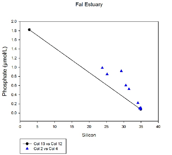
EC.9 where the introduction of the Fal River shows non-
Figure EC.9: Showing non-
All nutrients show increased concentrations towards the river end member, which is expected due to catchment geology and riverine inputs being a major nutrient source to the oceans (Bernard et. al. 2011). Differences in the Silicon and nitrate values at the river end members may be due to the different days the end members were collected on, over which rain fall increased; increasing weathering rates. However, it most likely due to anthropogenic causes such as agriculture and pollutants at the two different areas of the end members.
Dissolved silicon shows conservative behaviour. This is because the period in which the measurements were taken lays between the spring diatom bloom and the late summer siliceous dinoflagellate bloom, typically seen in the Western English channels and surrounding areas (Rodriguez et. al. 2000).
Phosphate, a limiting factor for most phytoplankton growth (Yool, Tyrrell, 2002),
shows signs of non-
Nitrate appears to act conservatively. This data shows that down the estuary there is no biological activity removing nutrients. As no large increases in nutrients are observed, it can be suggested that the smaller rivers leading into the estuary have little effect with respect to nutrient concentrations.
With a more detailed profile of the surface nutrient compositions in each river, a more conclusive study can be conducted as to whether the Rivers have any additions or removals. The major issue with the data is that station 4 samples were collected at the fork of the Truro and Fal River. As samples were taken on the flood tide, there is the possibility that some water from the Fal was transported up into the Truro River. This may also explain why the fresh water pockets were seen as the vessel approached the Fal River. To obtain a more reliable Truro end member, samples can be taken as the river approaches the Fal River, on the ebb tide.
References
Bernard, C. Y., Dϋrr, H. H., Heinze, C., Segschneider, J., Maier-
Boyer, J. N., Kelble, C. R., Ortner, P. B., & Rudnick, D. T. (2009). Phytoplankton
bloom status: Chlorophyll a biomass as an indicator of water quality condition in
the southern estuaries of Florida, USA. ecological indicators, 9(6), S56-
Deane, E. M., & O'Brien, R. W. (1981). Uptake of phosphate by symbiotic and free-
Hallegraeff, G. M. (1984). Species of the diatom genus Thalassiosira in Australian
waters. Botanica Marina, 27(11), 495-
Heip, C. H., Goosen, N. K., Herman, P. M. J., Kromkamp, J., Middelburg, J. J., & Soetaert, K. (1995). Production and consumption of biological particles in temperate tidal estuaries. Oceanography and marine biology: an annual review, 33.
King, F. D., & Devol, A. H. (1979). Estimates of vertical eddy diffusion through
the thermocline from phytoplankton nitrate uptake rates in the mixed layer of the
eastern tropical Pacific. Limnology and Oceanography, 645-
Kolber, Z. S., Barber, R. T., Coale, K. H., Fitzwateri, S. E., Greene, R. M., Johnson,
K. S., ... & Falkowski, P. G. (1994). Iron limitation of phytoplankton photosynthesis
in the equatorial Pacific Ocean. Nature, 371(6493), 145-
McAllister, C. D., Shah, N., & Strickland, J. D. H. (1964). Marine phytoplankton
photosynthesis as a function of light intensity: a comparison of methods. Journal
of the Fisheries Board of Canada, 21(1), 159-
Rodriguez, F., Fernandez, E., Head, R.N., Harbour, D.S., Bratbak, G., Heldal, M.,
& Harris, R.P. 2000. Temporal variability of virus, bacteria, phytoplankton and zooplankton
in the Western English Channel off Plymouth. Journal of the Marine Biological Association
of the United Kingdom. 80(4), 575-
Yool, A., Tyrrell, T., (2002). Role of diatoms in regulating the ocean’s silicon
cycle. Global biogeochemical cycles, Vol 17, No. 4, 1-
Webster, I. T., Smith, S. V., & Parslow, J. S. (2000). Implications of spatial and
temporal variation for biogeochemical budgets of estuaries. Estuaries, 23(3), 341-
Estuary
| Introduction |
| Methods |
| Results |
| Discussion |
| Physical |
| Chemical |
| Biological |
| Physical |
| Chemical |
| Biological |
| Introduction |
| Methods |
| Results |
| Discussion |
| Physical |
| Chemical |
| Biology |
| Physical |
| Chemical |
| Biology |