Falmouth Field Trip 2014- Group 3

This website reflects the opinions of students and not the views of the University of Southampton or the National Oceanography Centre.

Produced by: Alice Duff, Philippa Fitch, Joanna Gordon, William Harris, Thomas Jefferson, Eirian Kettle, Jesse Marshall, Dominique Mole, Emma-Jo Pereira, Joshua Walton

Estuary - Physical

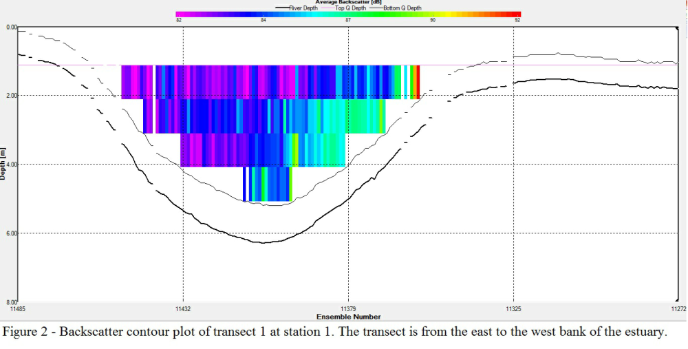
Station 1

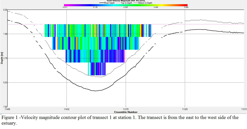
A change in backscatter can be seen across the transect of the estuary. This is due to a change in velocity affecting the amount of sediment suspended.  Transect 1 is located just after a meander in the estuary. As data collection was during an ebb tide, the flow was southward and the meander caused an increase in velocity to the eastern side and a decrease to the west. The decreased flow speed to the west will have also experienced eddies, increasing sediment suspension in the west. This explains the larger backscatter values seen here by the bed and sides of the estuary. See Figures 1 and 2 for velocity  and backscatter contour plots.

Station 2

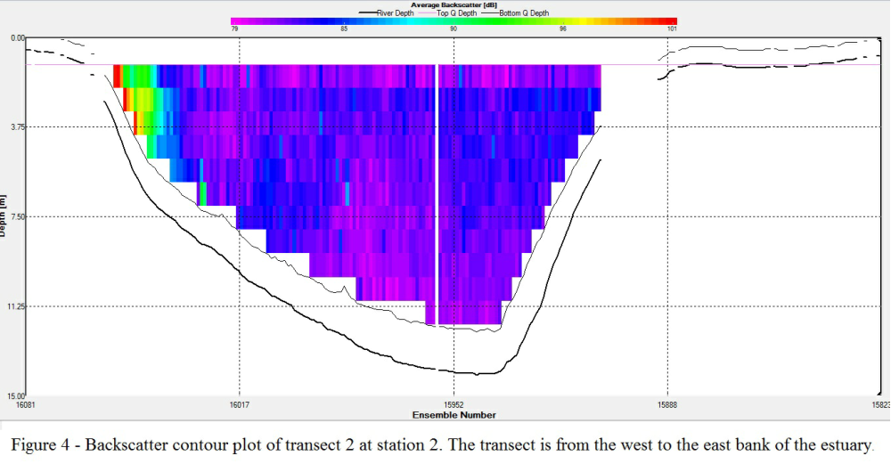
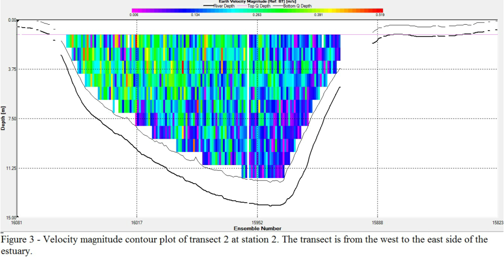
As this station is located just after the joining of two tributaries, flow speeds again vary along the transect. The amount of backscatter remains fairly consistent except for the far west bank of the estuary where a sudden increase is seen. This may be caused by the inside section of the meander where transect 2 is located. See Figures 3 and 4 for velocity and backscatter contour plots.

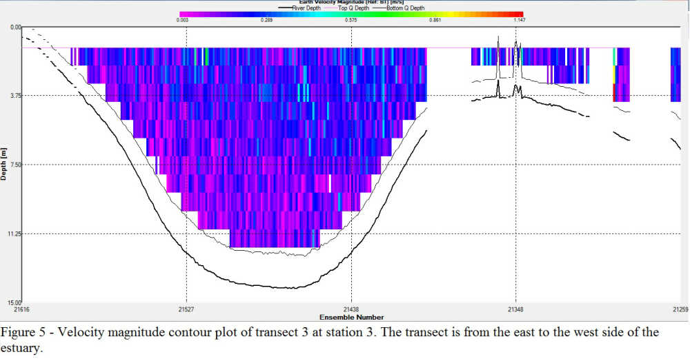
Station 3

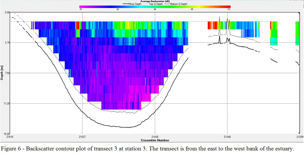
A uniform flow velocity is seen along this transect. The backscatter increase seen at the surface will therefore be a result of zooplankton grazing on phytoplankton in surface waters. See Figures 5 and 6 for velocity and backscatter contour plots.

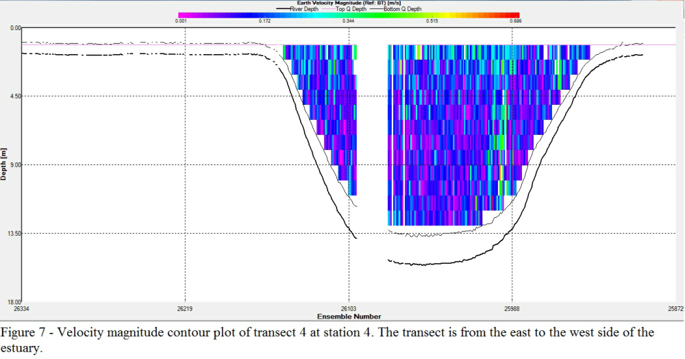
Station 4

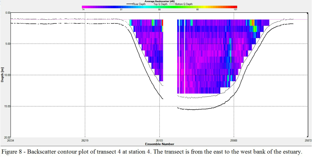
A section of data was missed on this transect. Although repeat transects were attempted, a technical malfunction with the ADCP meant we could not collect data for the whole transect. This problem persisted for the remainder of the transects. Both backscatter and velocity increase from the bottom to near the surface on the eastern side of the transect. Due to its small size it is likely to be an object in the water such as a mooring chain. The increase in backscatter at the surface is again due to zooplankton. See Figures 7 and 8 for velocity and backscatter contour plots.

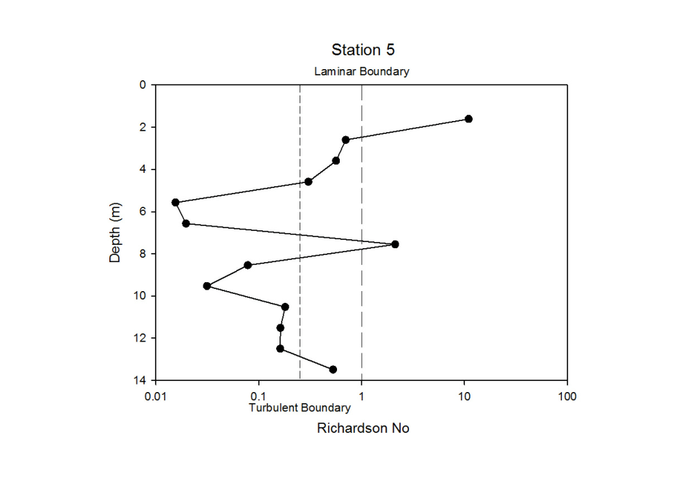
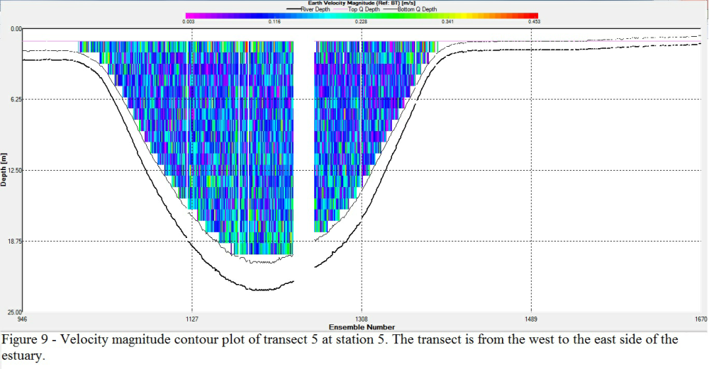
Station 5

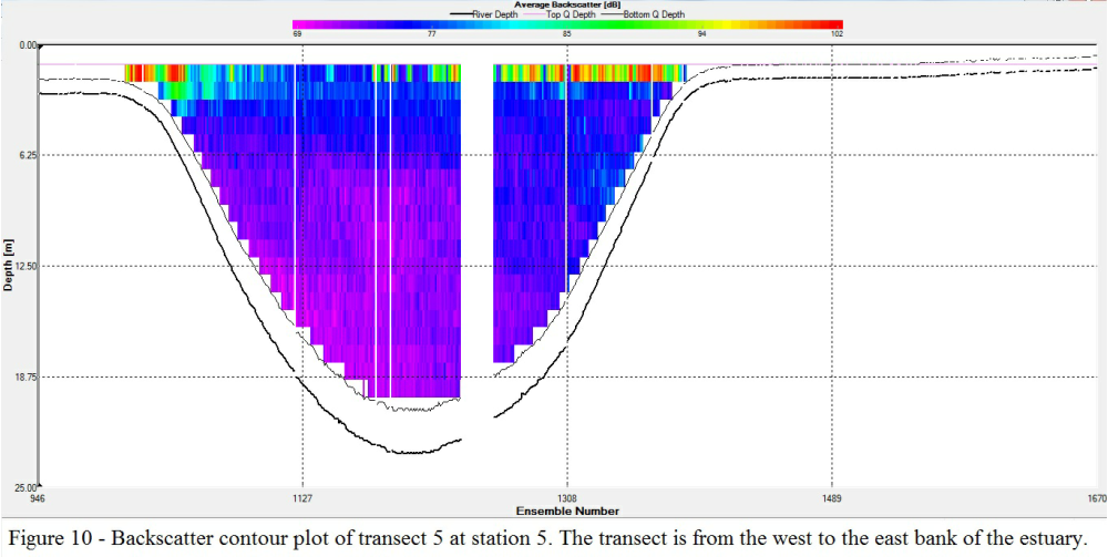
The velocity at this station shows large variations in very small spatial differences. This suggests mixing of the water is occurring and that it is very turbulent due to shear between each of the adjacent velocity differences. A large proportion of the estuary was missed in this transect due to the shallow water depth. Backscatter again increases at the surface due to zooplankton and remains constant throughout the rest of the water column. See Figures 9 and 10 for velocity and backscatter contour plots.

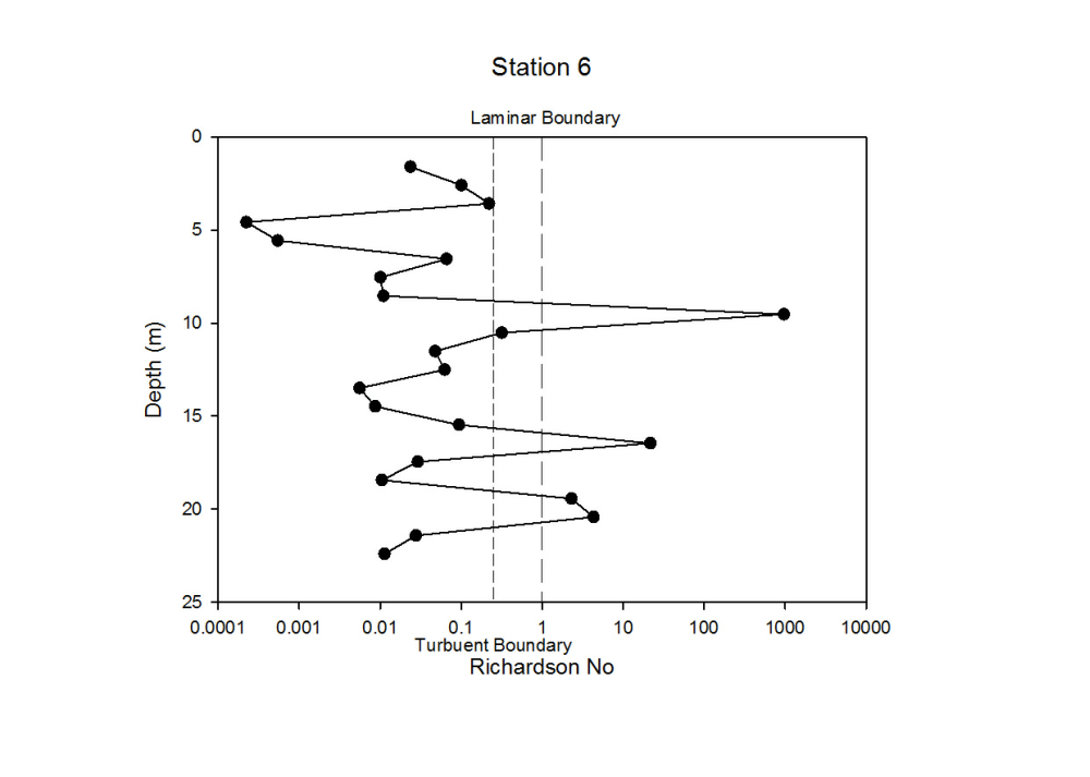
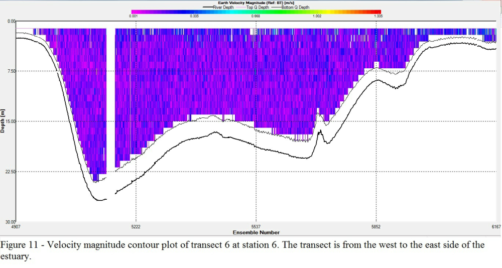
Station 6

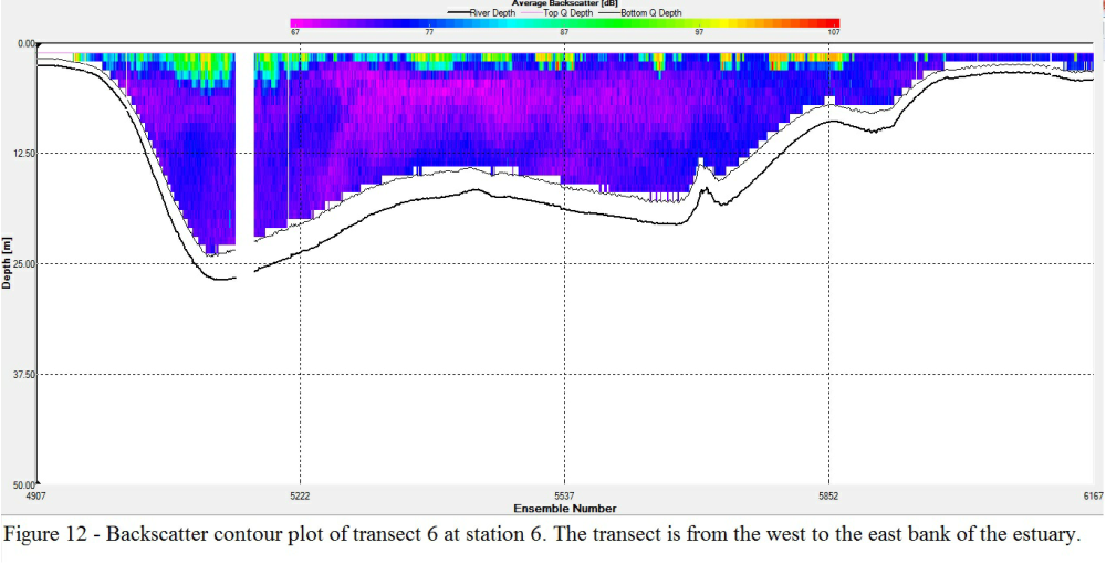
Flow velocity becomes more uniform again along this transect. The average flow speed also increases slightly compared with Station 5 even though it was sampled just before low tide when flow velocity should be slowing down. This may be due to the Stations increased proximity to the mouth of the estuary where it becomes deeper allowing greater flow speeds. The layer of zooplankton appears to be thickening compared with Station 5, shown by increased backscatter at the surface reaching up to 4m. See Figures 11 and 12 for velocity and backscatter contour plots.

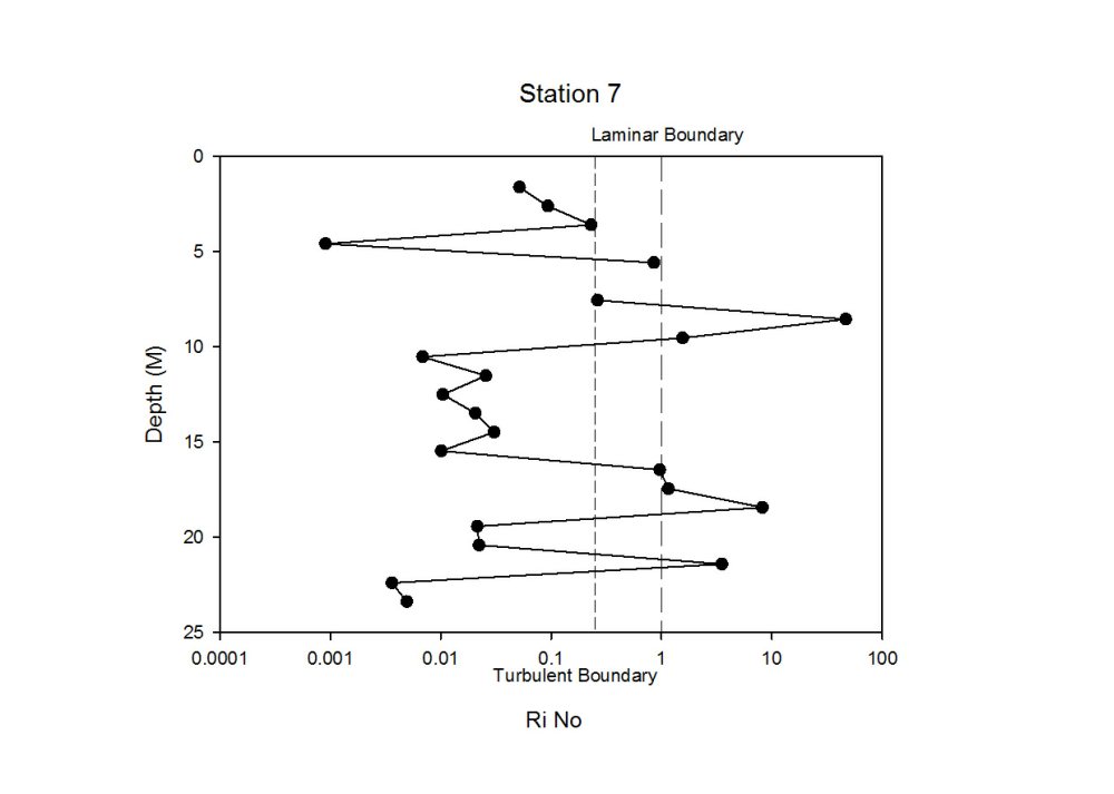
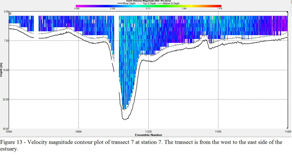
Station 7

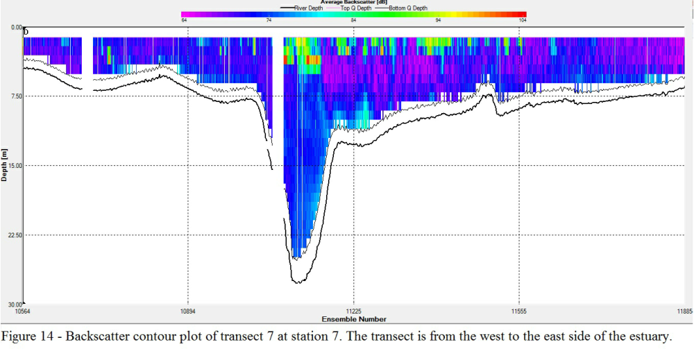
Taken at the widest part of the estuary, a significant depth change is seen across this transect due to a main channel in the middle of the estuary. Faster flow velocities are seen in this channel as expected due to the increased depth. An increased backscatter is also seen at the surface above this main channel and to the east where the estuary is deeper. Zooplankton caught in the flooding tide will have been transported into the estuary primarily through the main channel near the surface and may be the reason an increase in backscatter is only seen here. See Figures 13 and 14 for velocity and backscatter contour plots.

Temperature, Salinity and Density

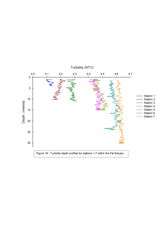
Turbidity

Results - Turbidity values increase from the head to the mouth of the estuary with the highest volts recorded at Station 7 (Figure 19). At all stations the vertical profiles are relatively homogeneous with depth. Station 1 had the lowest recorded voltage with values close to 4.1 throughout the water column. Stations 4 and 5 have very similar voltage recordings as do Stations 6 and 7. Station 7 had the highest recorded voltage with values close to 4.6. No turbidity maximum is seen on at any stations.

Discussion - Higher turbidity levels are typical found at the top of the estuary near Truro due to sediment input from rivers (Langston et al., 2006). However, low tide occurred when samples were collected at Station 1, hence, there was less tidal movement resulting in lower turbidity values. Falmouth estuary is a tide-dominated estuary and when sampling Stations 5-7 high spring tide was rising. These tidal currents at the seaward end caused strong mechanical mixing throughout the water column at these stations and this accumulation of suspended particulate matter created higher turbidity compared to stations at the top of the estuary. Station 4 was sampled as high tide had just started rising, suggesting  the effect of the tides on the results was small. Since it is a long estuary, this suggests it has reasonably long flushing time. Particles will therefore stay in suspension longer and accumulate at the mouth of the estuary (Uncles et al., 2002).

ADCP

Generally, greater flow speeds are seen further down the estuary. This is to be expected due to an increase in depth meaning less friction acting on the flow. The mixing within each transect also increases down the estuary, although a number of topological factors increase mixing and sediment suspension at Stations 1 and 2. By Station 3, any backscatter increase is primarily a result of zooplankton in surface waters but care was taken to ensure no anomalies in surface zooplankton came about from the vessel being underway. This can cause bubbles to pass over the ADCP probe on the hull of the boat and cause false backscatter (Heywood et al, 1991). Individual factors influencing flow velocity and backscatter are discussed below with figures for each station.

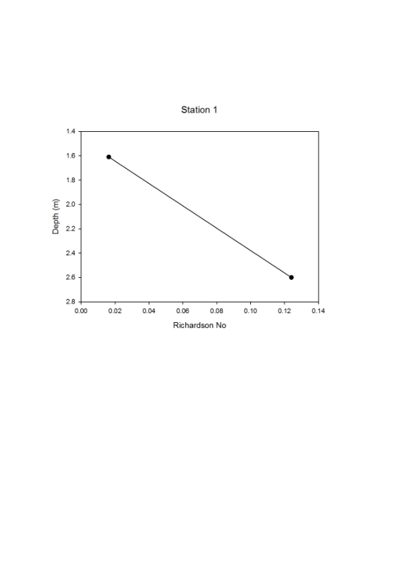
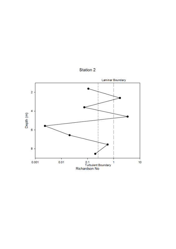
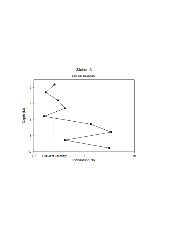
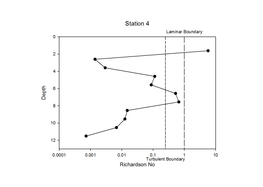
Richardson’s Number

A comparison of the overall profiles of all the stations shows that the majority of the water column experiences turbulent flow (Figure 15). This is shown by the Richardson number calculated at the sampled depths having a value less than 0.25, indicating turbulent flow while there are also Richardson values greater than 1.0 around the thermocline.

Overall, the low Richardson number (Ri No.) and the corresponding turbulent flow in the water column indicates that the estuary is well mixed. This is supported by T/S measurements taken using the CTD at each of the stations which show that Falmouth estuary is a tidally dominated estuary as the water column is mixed with little or no halocline (Segar, 1998). Corresponding salinity profiles for the 7 stations are important in interpreting the Ri No. observed. Stations 1 and 2 in the upper estuary have lower Ri No. and more turbulent flow than further down the estuary because there is greater shear due to the decreased depth and narrower channel. Station 3 is unusual in that it displays significantly higher Ri No. values than Stations 1 and 2 but also greater than the stations further down the river. This is due to the location of Station 3 being in the outflow area of additional sources of fresh water (Cowlands and Lamouth Creek) that creates a warm fresh upper layer, leading to higher Ri No. causing stratification and the formation of a weak halocline.

Mixing is a gradual process and the water becomes more mixed as it goes downstream even though the average Ri No. is increasing, indicating less turbulent flow. This is despite the fact that velocity increases slightly as you go further down the estuary due to the increased depth. The salinity/depth plot illustrates this with salinity gradient at the upstream stations becoming linear from Stations 1-7. By the time the water gets to Station 7, there is no halocline with uniform profiles for salinity and temperature throughout the water column.

Figure 15 - Richardson number profiles for Stations 1-7. Click figures to enlarge

Click figures to enlarge

Temperature contour plot

Figure 16 shows that the temperatures are highest in the surface water. At Station 1, the highest value is ~18.5°C. The lowest temperatures were found in the bottom water at Station 7, the lowest temperature was ~17.0°C. As you move down the estuary, from Station 1 to Station 7, the general trend shown is a decrease in temperature. This temperature decrease is not limited to the surface waters but occurs at all depths.

Salinity contour plot

The lowest salinity recorded was at the surface of Station 1. This is expected as it is the most freshwater station, being highest up the estuary (Figure 17). From here a continuous increase in salinity is seen, relatively uniform with depth across each station. The biggest change in salinity is between Stations 3 and 4 where a 0.5 PSU change is seen. This suggests the position of a riverine and seawater boundary. Some slight undercutting of freshwater by seawater is seen further down the estuary as a result of the increased density due to higher salinities of the seawater.

Density contour plot

The density contour plot, Figure 18, shows there is little change in density seen in the depth profiles from each station when viewed alone. However, when together in the plot an increase in density can be seen in the horizontal plane as you move from Station 1 to 7. This increase is caused by the decrease temperature and increase in salinity discussed previously.

Click figures to enlarge

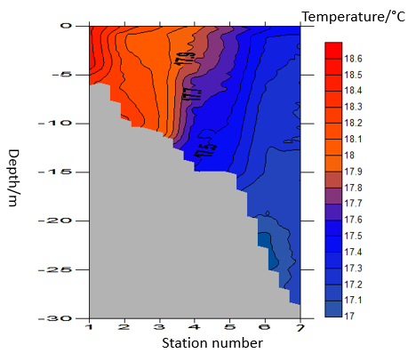
Figure 16

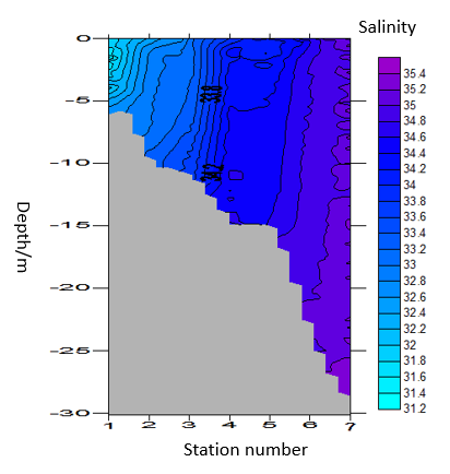
Figure 17

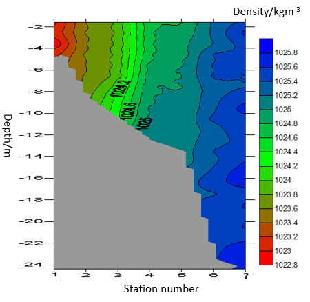
Figure 18

Click figure to enlarge