Falmouth Field Trip 2014- Group 3

This website reflects the opinions of students and not the views of the University of Southampton or the National Oceanography Centre.

Produced by: Alice Duff, Philippa Fitch, Joanna Gordon, William Harris, Thomas Jefferson, Eirian Kettle, Jesse Marshall, Dominique Mole, Emma-Jo Pereira, Joshua Walton

Locating the Fronts

Offshore - physical

ADCP

Richardson Number

Temperature, Salinity, Density and Turbidity

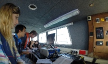
The aims of the offshore practical were to determine and identify the physical structures of the water column. The temperature and salinity of seawater at 1m depth were used to locate fronts in order to do CTD profiles of the water column. Station 45 displayed characteristics of an estuarine front due to its location and large, shallow thermocline. Temperature and salinity were monitored continuously while between 12:20 and 12:25 UTC. Increasing temperature and salinity was observed (Figure 1), determining the position of Station 48 as this suggested a the presence of a front. A CTD profile was carried out but the water column was found to be still well mixed. This suggested stratification had not fully occurred as expected.

The CTD at Station 49 was deployed at 13:13 UTC when temperature increased indicating a front. Again, soon after the CTD was launched, temperature and salinity reduced indicating that a front had still not been located. The CTD depth profile showed some stratification of the water column. At 13:50 UTC was there a large increase in temperature to 17.75°C, again indicating the location of a front. The CTD was launched at 14:10 UTC and the depth profile showed a stratified water column confirming our assumption as there was a warm water mass overlying a cold one (See Temperature Profile).   

Station 45/46

A layering of different backscatter values can be seen with depth. There are few high surface values which are likely to be due to bubbles under the hull of the boat. A more consistent value is seen just below the surface which proceeds to decrease at around 18m.The next layer of less backscatter remains until 35m where it continuously increases to the seabed. Flow velocity remains constant throughout the water column and some small sections of data deeper than 20m were missed when the boat was underway manoeuvring.

Station 47

There are areas of high backscatter in the surface waters shown in the backscatter transects for station 47. Once again these high values may be associated with interference from the boat. At greater depths the deployments from the rear of the Callista (CTD, zooplankton nets) can be shown by the higher values at depth. Surface waters also show higher flow velocities than bottom water.

Station 48

The backscatter transect for this station shows similar trends of inference from the boat and equipment as mentioned for the previous station. The velocity transect for this station is made up of patches of different velocity magnitudes,. This implies there is strong mixing in these areas with a high amount of turnover.

Station 49

A very uniform backscatter is also seen at this station with the various features being due to the interference from the boat rather than the water. The flow velocity is much slower at this station, as the previous station experienced flows greater than 1m/s in some places. There is lots of shear still occurring, shown by the vastly different velocity readings between each ADCP reading.

Station 50

In the upper 20 metres there is further ship related interference. The velocity transect shows that some of the deeper parts were not sampled due to limitations in the range of the ADCP. In the part of the water column that was sampled there is an increase in mixing compared to the rest of the transect .  

The Richardson Number (Ri No.) depth profiles were created using ADCP data taken at each station whilst sampling. As can be seen by the figures (below), all stations showed dominantly turbulent flow (<0.25 Ri No.) which was to be expected given all locations were in the tidally dominated English channel. Stations 47-49 were also located just off Lizard Point, a headland that marks the edges of 2 bays. This is likely to produce exceptionally turbulent waters due to back eddies from different flow directions out of the two bays. Station 47, being closest to the headland showed the most turbulent waters and also the most well mixed water as seen in our CTD depth profiles.  

The line of best fit at Station 48 and 49 (Figures 20-21) show a slight increase in Ri No. closer to the surface. No depth below 33m shows laminar flow in either plot each of which is 60m deep. This could show some of the turbulence caused by the headland and mark a ‘Surface’ front. Bottom fronts are dominated by wind stirring and surface fronts by tidal effects (Pedersen, 1994). It is believed to be caused by tides rather than wind due to the headland causing eddies. The maximum depth of ADCP reading was 53m whilst true depth at these stations was 70m. The trend of increasing turbulence in flow may have continued right to the seabed but this cannot be fully concluded as data collection at these depths was not possible.

An occasional very high Ri  No. is seen at some stations, for example the shallowest reading at Station 48. These are likely to be anomalies due to false backscatter from objects in the water.

Click the figures below to enlarge and see  a short discussion for each station.

A layering in backscatter was seen at the stations that were identified to have fronts present (stations 45/46/50); this is likely to be due to their interactions between the converging water masses with differing quantities of suspended particulate material. The other stations showed more uniform backscatter associated with their well mixed profiles. The expected trend between flow velocity and backscatter was observed as they were in reverse to each other. The stratified water columns demonstrated more laminar flow., whereas those that were well mixed showed turbulent flow.

Click Figures to enlarge

Density increases with depth, therefore the deeper stations such as Station 45 (60.5m) show the highest density reading (1026.85kgm-3). Density increases as distance from the coast increases. This phenomena is be due the frontal system at Station 45. This body of warmer water is less dense than the underlying colder water. There is an increase in turbidity (transmission) at the front due to the well mixed surface layer. This turbidity decreases at depth and distance from the frontal system as the water movement decreases. At Station 50, there is also a frontal system present, shown be the rise in surface temperature and decrease in density in the first 10m.. Throughout the water column, at Station 50, there is a slight increase in turbidity . Salinity is fairly uniform throughout the stations with a slight decrease at Station 47.  (See figures 23-26 below)

Click figures to enlarge