ESTUARY RESULTS

AND DISCUSSION

Results:

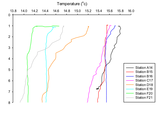
Figure 1 demonstrates the changes in temperature (ºC) with increasing depth (m), over eight stations. All sampled stations display an overall decrease in temperature from the surface measurement to the deepest depth of 8m (except A14, which reached 7m as the greatest depth). Station A14 displays the highest surface temperature (15.8 ºC) whereas station E19 shows the lowest recorded surface temperature (14.6 ºC). Station D18 shows the most dramatic decrease in temperature, declining from 15.2 ºC to 14.3 ºC, whereas station B15 indicates the most linear trend, with a small decline from 15.7 ºC to 15.5 ºC.

Discussion:

Temperature followed the expected trend: to decrease with depth. This is primarily due to the stratification of the water column, whereby fresher, less saline water overlies the denser, more saline water. Therefore, the denser water absorbs less heat energy as denser water takes more time to absorb energy. Additionally, as the denser water sinks, it is less able to obtain heat due to the attenuation of light with depth. Temperature changes along the course of the transect, from station A14 to G21. A14 displayed the highest surface temperature, as this station was situated furthest up the estuary (towards the river), the temperature was highest because bodies of riverine water have a less volume and a lower surface area, meaning that less energy is needed to heat the water. On the other hand, seawater is expected to have a lower temperature, due to the greater volume and higher surface area, meaning that more energy is needed to heat the surface body of water. Therefore, temperature declines from the station nearest the river (A14) to the station nearest the sea (G21).

Figure 1. The thermal structure of the water column, measured using the CTD at each of the 8 stations.

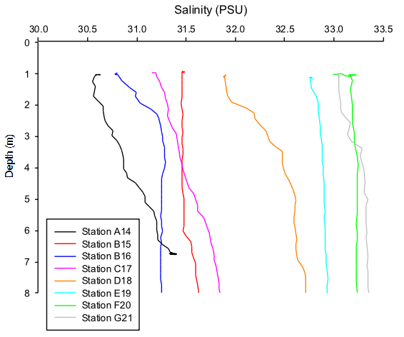
Figure 2. The salinity structure (PSU) of the water column, measured at various stations throughout the Fal estuary.

Results:

Figure 2 exhibits the changes in salinity (PSU) with increasing depth (m), over eight stations. All stations show an overall increase in salinity with depth, from the surface measurement to the deepest depth of 8m (except A14, which reached approximately 7m as the greatest depth). Station G21 displays the greatest surface salinity reading (33.1 PSU), whereas station A14 shows the lowest salinity recorded at the surface across all stations (30.6 PSU). Both stations A14 and D18 indicate the greatest rate of change from the surface salinity to the salinity at depth (A14: 30.6 – 31.4 PSU and D18: 31.8 – 32.7 PSU). Station F20 shows the least change in salinity with increasing depth, with a highly linearized pattern, increasing from 32.9 PSU to 33.2 PSU (0.3 PSU change).

Discussion:

Salinity is shown to increase with subsequently increasing depth. This is primarily due to the freshwater being sourced from the river, possessing an overall lower salt content, therefore the freshwater is less dense than the high salinity seawater. This leads to the freshwater overlying the seawater layer in the water column, as the denser seawater will sink. This produces the expected salinity profile.

Figure 3. Estuarine mixing diagram showing the X  behaviour of silicate. Theoretical Dilution Line (TDL) connects the river endmember to the marine endmember.

Figure 4. Absorbance of known concentrations of silicon, used to calculate concentration from values of chlorophyll  bsorbance taken from samples.  

Results:

Fig. 3 indicates the relationship between salinity (PSU) and silicon concentration (µmol/litre silicon), with a Theoretical Dilution Line (TDL) joining the river endmember (River Allen) to the marine endmember, displaying a negative linear relationship. Salinity increases from the riverine endmember to the marine endmember, whereas silicon concentration decreases as salinity increases. Non conservative behaviour is shown as the data points lie to the removal side of the TDL (below), therefore silicon is removed from the estuary at this point.

Figure 4 displays a silicon standards chart, in the form of silicon concentration plotted against absorbance which has been blank corrected; this essentially means that any absorbance detected from the 0.0 µmol/l silicon concentration was taken off of every other absorption measurement, bringing all the data down to calibrate for residual absorbance by the spectrophotometer (which should display 0 absorbance for 0.0 µmol/l silicate concentration). Figure 4 has plotted concentrations of silicon from 0 – 10 µmol/l and their relative blank corrected absorbance values. The relationship is positively linear, meaning as silicon concentration increases in the sample, so does absorbance.

Discussion:

Salinity is shown to increase with subsequently increasing depth. This is primarily due to the freshwater being sourced from the river, possessing an overall lower salt content, therefore the freshwater is less dense than the high salinity seawater. This leads to the freshwater overlying the seawater layer in the water column, as the denser seawater will sink. This produces the expected salinity profile.

 Silicate

 Phosphate

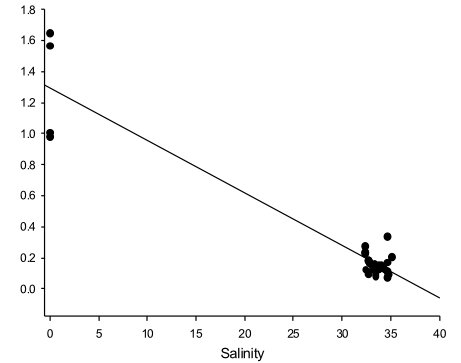
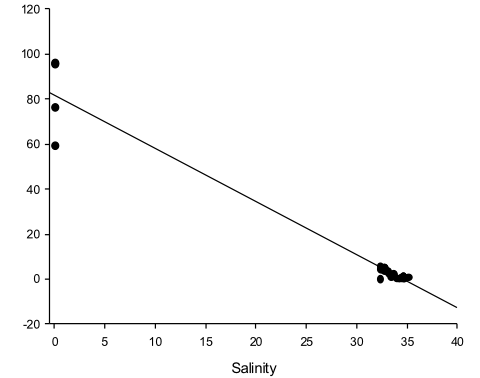
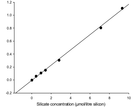
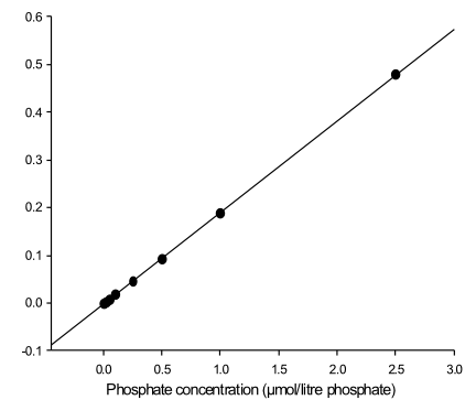
Figure 5. Estuarine mixing diagram showing the X  behaviour of phosphate. Theoretical Dilution Line (TDL) connects the river endmember to the marine endmember.

Figure 6. Absorbance of known concentrations of phosphate, used to calculate concentration from values of chlorophyll  absorbance taken from samples.  

Results:

Fig. 5 indicates the relationship between salinity (PSU) and phosphate concentration (µmol/litre phosphate), with a Theoretical Dilution Line (TDL) joining the river endmember to the marine endmember. A negative linear relationship is shown between the two endmembers, whereby salinity increases with decreasing phosphate concentration. Phosphate illustrates non conservative behaviour, due to the majority of the data points lying below the TDL, further indicating removal from the estuary (despite one point lying above the TDL).

Figure 6 displays a phosphate standards chart in the form of concentration plotted against absorbance, which has been blank corrected (as previous). Figure 6 has plotted concentrations of phosphate from 0 – 3 µmol/l and each relative blank corrected absorbance values. The relationship is positively linear, meaning as phosphate concentration increases in the sample, so does absorbance.

Discussion:

Bioreactive phosphate is removed from the estuary by phytoplankton, as it is used in many cellular processes, such as respiration and photosynthesis (Morris, Bale and Howland, 1981). The non-conservative behaviour is likely due to said removal, as the spring bloom will have finished and low nutrient concentrations will be expected until upwelling events during the winter (Prego et al, 2007). Phosphate can also be absorbed by particulate materials, which would account for increased removal in the upper estuary (Bale and Morris, 1981).

 Nitrate

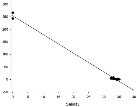
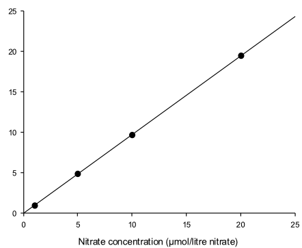
Figure 7. Estuarine mixing diagram showing the X  behaviour of nitrate. Theoretical Dilution Line (TDL) connects the river endmember to the marine endmember.

Figure 8. Absorbance of known concentrations of  nitrate, used to calculate concentration from values of chlorophyll  absorbance taken from samples.  

Results:

Fig. 7 indicates the relationship between salinity (PSU) and nitrate concentration (µmol/litre nitrate), with a Theoretical Dilution Line (TDL) joining the river endmember to the marine endmember, showing a steep negative gradient, indicating a strong negative linear relationship between the two parameters (as salinity increases, nitrate concentration decreases). Along with silicate and phosphate, nitrate displays non conservative behaviour, indicated by the data points lying below the TDL.

Figure 8 displays a nitrate standards chart, in the form of concentration plotted against absorbance. These absorbance values have been blank corrected to remove residual absorption (as previous). Figure 8 has plotted concentrations of nitrate from 0 – 25 µmol/l and each relative blank corrected absorbance values. The relationship is unsurprisingly positive and linear, meaning as nitrate concentration increases in the sample, so does absorbance.

Discussion:

Nitrate can exhibit several different behaviours in an estuary, however non-conservative behaviour can be due to different things. Uptake by phytoplankton for biological processes such amino acid and protein production, and DNA synthesis (Iyengar, Stuehr and Marletta, 1987). However, nitrogen can also be removed by conversion to gaseous forms and sediment burial (Gardner et al, 2006) which could be why it appears non-conservative, as the spring bloom is over so less nitrate is being removed.

 Phytoplankton

Results:

The speciation of phytoplankton sampled from surface waters change across the length of the Fal estuary. Chaetoceros spp. initially shows a decrease in abundance as sampling progressed from station A14 to C17; none appear to be present at site D18 however, thereafter, their abundance begins to increase again to levels that were greater than they initially were at the top of the estuary. Throughout the entire length of the Fal estuary sampled, Skeletonima were the most abundant species, numbers per 10ml however, decreased between stations E19 and G21. Leptocylindrus were documented at sites A14 and B15 but no recording were made thereafter. Comprenos spp. were present only at station D18 whilst Landeria spp. was sampled only at G21. Note that only 6 phytoplankton samples were taken and therefore, station F20 has no recoding of the species present.

Discussion:

The occurrence of Comprenos spp. and Landeria spp. at a single site within the Fal estuary could be either a result of false identification or that organisms were actually only present at these stations. To verify this, it would require repeat sampling of the area under investigation.

Chaetoceros spp appears to have distributions that are unaffected by salinity. The increase in numbers per m-3 on either side of station D18 would rule out salinity being a limiting factor, as there would be no Chaetoceros in the upper estuary if the salinity is too low. Therefore, the distributions of Chaetoceros spp is more likely due to levels of nutrients or to grazing by zooplankton, but that would need to be verified by further sampling and observation.

Skeletonema (Figure 10) is a diatom that occurs in both marine and brackish waters (Balzano, Sarno, Kooistra, 2010). Although high concentrations per m-3 were found, there appears to be no overall trend. In order to discover one, repeat sampling would probably be required.

Zooplankton

Discussion:

The relationship between adult copepods and juvenile copepods in the naupliar stage could be attributed to the observed cannibalistic behaviour between adult individuals and the juveniles. This has been quantified in several different studies, with values for percentage of naupliar larvae cannibalised ranging from 35% in the North Sea (Daan, Gonzalez, and Klein Breteler, 1988) to 99.5% in tanks used for domestic rearing of copepods (Drillet et al, 2011).

It is important to add that many species of copepod are cannibalistic both to their own species and to other species (Bonnet, 2004), which makes it more likely that the pattern observed is due to general predation of copepod species on copepod nauplii.

The increase in adult copepod concentrations could be attributed to their increased tolerance to lower salinity levels (Lance, 1963), whereas juveniles have better survival rates at higher salinities (Chinnery and Williams, 2003).

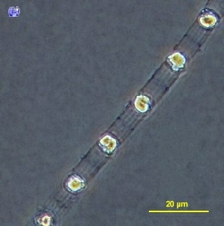
Figure 10. Skeletonema with a scale bar for size reference. Image courtesy of  planktonnet.awi.de. Available from: https://planktonnet.awi.de/index.php?Contenttype=image_details&i temid=55195 [Accessed 01/07/16].

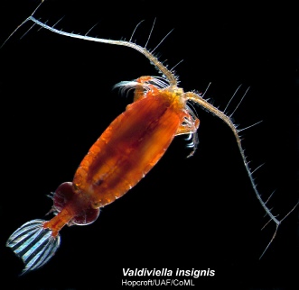
Figure 12. Common copepod V. insignis. Image courtesy of The Copepod Project. Available from: https://www.st.nmfs.noaa.gov/copepod/about/index.html

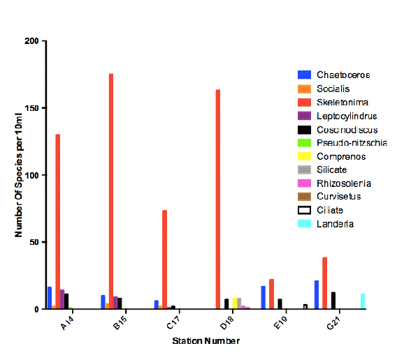
Figure 9. Total number of each different Phytoplankton species found per 10ml water sample counted under a light microscope, for stations A14, B15, C17, D18, E19 and G21 (increasing distance down the estuary from the river end to the seawater end) sampled from a Niskin bottle on the RV Bill Conway. The most abundant species present in every station sampled was Skeletonima (most abundant at station B15 – 175 individuals per 10ml). There were a fair few species found only at a single sample station also; Pseudo-nitzshia present at A14 only, Comprenos, Silicate, Rhizosolenia and Curvisetus all present only at station D18, Ciliate present at E19 and Landeria present only at site G21.

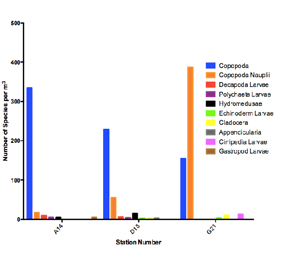
Figure 11. Number of individuals of each species of Zooplankton (per m3) within stations sampled on the RV Bill Conway (A14, D18 and G21). These stations were from the river end of the estuary (A14), to the middle of the estuary (D18) down to the seawater end of the estuary (G21). There are two main trends seen in this graph; Copepoda numbers per m3 decrease with distance down the estuary, whereas Copepoda Nauplii increase with distance down the estuary, from the river to seaward end.

The views and opinions expressed on this website are those of individuals within group 8 and are not associated with The National Oceanography Centre, University of Southampton or Falmouth Marine School.