

Method:
100ml surface water samples were collected from a Niskin bottle and stored in a glass bottle containing 1ml of Lugol’s iodine solution to preserve and stain the phytoplankton. In the lab, the 100ml solution was reduced to 10ml and stored in a glass vial. Pipetting was used to place the solution on a Sedgewick rafter cell, allowing us to obtain data from 100µl of the solution. The data obtained was a count of different genuses and a total of phytoplankton cells, which was multiplied by 10 to get a representation of how many cells were in 1ml of the solution.
Method:
We used a net with a 200µm mesh and a 50cm diameter connected flow meter and a 1L bottle to collect the zooplankton. The net was towed behind RV Bill Conway, for each sample latitude and longitude for the start and end was recorded, number of flowmeter revolutions for the start and end was recorded and the time at the start and end was recorded. Once the net had been recovered, the seawater containing zooplankton was transferred to another bottle and then fixed with 10% formaldehyde solution.
The sample was inverted to mix, and 10ml was measured from the 1L zooplankton sample, using a measuring cylinder. 5ml of this was pipetted into a Bogorov tray, and the zooplankton were counted and identified under stereo microscope. This was repeated with the remaining 5ml. Calculations were then used to obtain zooplankton per 1m3 of seawater.
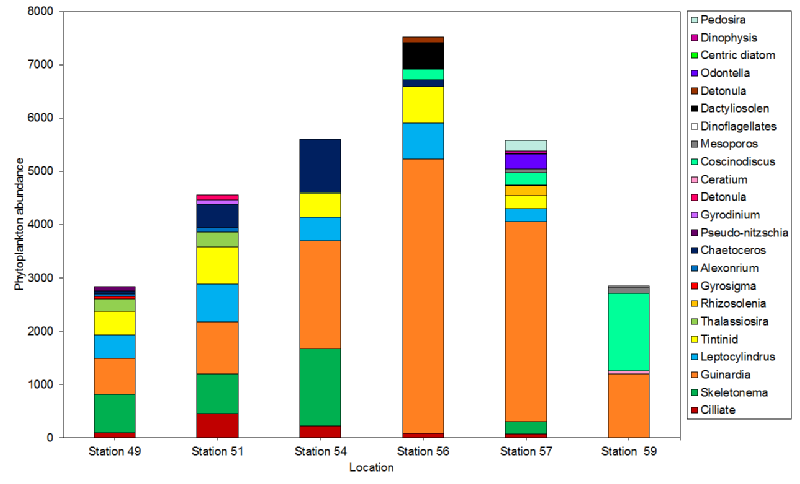
Figure 14: Stacked bar graph of the abundances of different phytoplankton groups at six different stations along the Fal Estuary on 27/6/16 between 08:30 and 14:40 UTC.
Station 56 had the highest overall abundance of phytoplankton at around 7500 specimens, followed by Stations 54, 57, 51 and then Stations 49 and 59 had the lowest overall abundances at less than 3000 specimens. Station 59 has the lowest phytoplankton diversity as well as low abundance, and Station 49, although it has low abundance, has high diversity. Stations 51 and 57 have middling phytoplankton abundance and high diversity, with Station 56 having less diversity even with the highest abundance, and Station 54 has the lowest abundance after Station 59.All stations have a large number of Guinardia, although they are especially abundant at Stations 56 and 57. Skeletonema was of nearly equal numbers to Guinardia at the first three stations, and Conscinodiscus had a larger abundance than Guinardia at Station 59. All stations except 59 contained Tintinnids and Leptocylindrus. Station 54 has the highest number of Chaetoceros, followed by Station 51, 49 and 56, with 57 and 59 having none. Station 56 is the only station to contain Dactyliosolen and has them in similar numbers to Leptocylindrus.
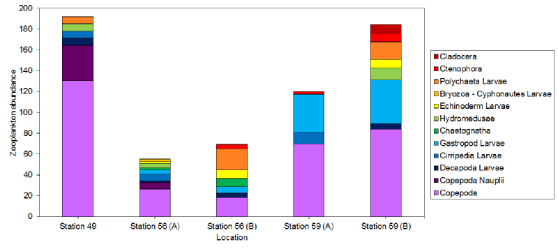
Figure 15: Stacked bar graph of the abundances of different zooplankton groups at three different stations along the Fal Estuary on 27/6/16 between 08:30 and 14:40 UTC. Station 49 only has one set of abundances and Stations 56 and 59 have two sets of abundances.
Station 49 has the highest overall abundance, followed by station 59, although the second set of calculations has a higher abundance than the first by about 70 specimens. Station 56 has the lowest abundance overall. Station 56 has the highest diversity of zooplankton, even when averaged over the two calculations. Station 59A has the lowest diversity, although 59B has the highest diversity after Station 56. Station 49’s diversity lies between 59A and 59B. However, the difference in the calculations within Stations 56 and 59 leaves room for speculation about true abundances. All stations contain a large proportion of copepods in their overall abundance, with Station 49 having the highest abundance of copepods, followed by Station 59 and with Station 56 having the lowest copepod abundance. In terms of Copepod nauplii, Station 49 has the most, Station 56 only has a small amount in one of the calculations, and Station 59 has none. Station 59 has the largest amount of Gastropod larvae, with Station 56 not having much and Station 49 having none. All stations appear to have some bryozoans, but only in the second set of data. These only amount to a small proportion of the overall abundance, except at Station 56, where they have a greater abundance than copepods.
Glass bottles were filled with water samples from the Niskin bottles, and the samples were fixed using by adding the following reagents – 1ml Manganous Chloride solution and 1ml of Alkaline Iodide solution. The bottles were inverted to mix, and stored in a bucket of water to prevent accidental oxygen exchange. One measurement of dissolved oxygen was taken per station at different depths, so we could not analyse the results as there was insufficient to draw conclusions.
The syringe was flushed using a small portion of the water from the sample bottle taken from the Niskin bottle. After flushing, 50ml of sample was loaded into the syringe and a filter was attached. The sample was slowly passed through the filter by depressing the syringe. The filter paper was removed from the filter and was placed into a test tube prepared with 6ml acetone solution. 3 replicates were taken from each sample, from the 3 depths sampled per station. A total of 36 samples were taken.
After having stored the samples of chlorophyll overnight in a dark freezer, they were analysed in the lab using a fluorometer. These fluorescence values were recorded and corrected to get an actual chlorophyll concentration using the following equation:
[((volume of acetone (6mls) / volume of seawater (50mls))] x fluorescence reading.
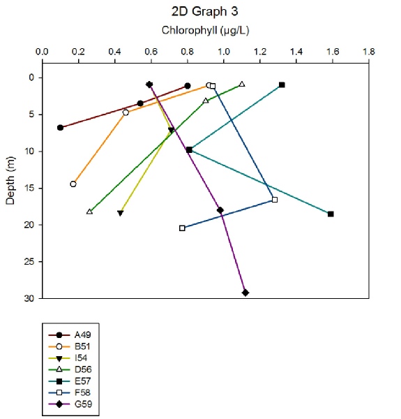
For sites closest to sea, Stations G59, F58 and E57, there appears to be deep chlorophyll maximums at around 15 to 20m depth. However chlorophyll concentration continues to increase down to 30m for G59, which is likely to be an anomaly. The rest of the sites further up the estuary show a general decrease in chlorophyll concentration with increasing depth. This could be due to the higher turbidity levels here, caused by shallower water and higher turbulence, thus reducing the depth at which light can penetrate.
Figure 18: A depth profile of chlorophyll from stations A49 - G59.
| Physics |
| Chemistry |
| Biology |
| Niskin |
| Flow meter |
| Light meter |
| Exosonde |
| Discussion |
| Physics |
| Chemistry |
| Biology |