Disclaimer: the views and opinions expressed are those of Group 9 members and not necessarily those of the University of Southampton, National Oceanography Centre or Falmouth Marine School

To attain the data, four pieces of equipment were deployed, a CTD rosette with Niskin bottles, an ADCP, a plankton net, and a secchi disk.

Most of the information on the physical properties of the water column would be collected using the CTD which was attached to the rosette with six Niskin bottles. When each station was reached (Station 13, 14, 15) the location, time and maximum depth was recorded. When we were ready the deck crew deployed the CTD with instructions from those working in the dry lab. As the CTD descended into the water column it recorded and sent the live data to the server in the dry lab where it was placed onto a graph. Just before the CTD reached the maximum depth it was stopped. The dry lab team used the information on the graph to decide where the niskin bottles should be closed for chemical analysis. The CTD was brought back to the ship repeating the recordings. This information was then saved for later analysis. For analysing the physical properties, the CTD had recorded temperature, salinity, turbidity, density, and irradiance. To add to our understanding of the levels of irradiance, we also used a secchi disk to work out the secchi depth. Data from the ADCP was used to calculate the Richardson’s number in order to understand the mixing taking place in the water column. The ADCP was also used observe the backscatter in the water.

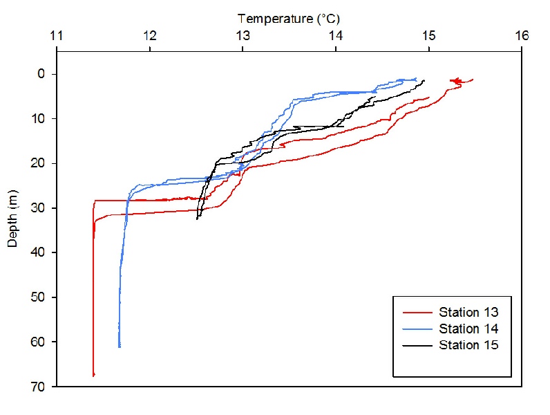
Initial analysis of the temperatures of the different station already starts to show a difference in structure in the offshore sites compared to the more inshore sites. As figure 1 shows, the water column is more stratified at Station 13 (red) with a clearly defined thermocline at 28.5m with a decrease from 12.7°C to 11.4°C, as well as this there is also a second thermocline visible at this station (though not as sharp) at 17m. Station 14 has a similar structure but the thermocline is not as well defined and is present at a shallower depth (25m), a slight second thermocline is also present but it is not as clear as the one present at Station 13 and is much closer to the surface. At Station 15, the most inshore and shallow site, the water column is more mixed with no clear thermocline, instead a gradual decrease in temperature between the surface and 20m from 14.9°C to 12.5°C at the seafloor. The double thermoclines at the offshore stations could be caused by localised warming at the surface paired with sea surface mixing caused by wind movement as well as the lack of mixing in these areas like is some other forms of thermoclines (Fiedler 2010).

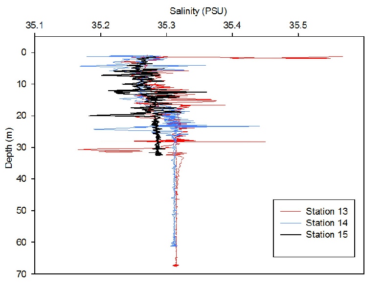
The salinity values vary far less than the temperature with all the station’s value between 35 and 36. Figure 2 shows many spikes in the data however this is more likely due to temperature lag in the sensors rather than any physical changes in the water (Horne and Toole 1980). The small variance in the salinity is similar at both Stations 13 and 14 with an increase in the salinity between the depths of 15m and 19m of 0.07. The salinity at Station 15 varies even less with a gain of 0.02 salinity at the seafloor. This is because more mixing is present at Station 15 so there will be little variance of salinity between and water bodies whereas at Stations 13 and 14 had some variance as a front was present.

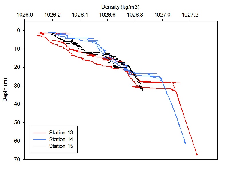
The density of the water column is a good indicator for the interaction of the main water bodies present in the water columns. The results are similar to the inverse of the temperature data. Figure 3 clearly shows depths where there is a rapid change in density of the water. These changes correspond to the thermoclines in figure 1 and show the stratified nature of Station 13 and 14 with a small amount of variance within each water body due to pressure but little to no mixing between water bodies. Like with the temperature, Station 15 shows an increased amount of mixing taking place throughout the whole water column with no pycnocline present.

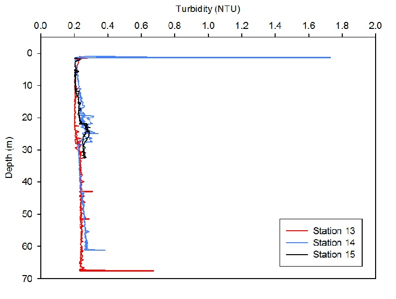
The turbidity data from the day supports the other data and could have been predicted based on the day. The weather was very calm over the whole day causing little movement in the water. The largest increases in turbidity take place at the surface of the water, at the air water interface, and on the sea floor where the water interacts with the sea floor. Other than this the only other changes in turbidity take place after 20m at Stations 14 and 15 (figure 4) though these changes are minimal (0.05). At Station 14 the increase in turbidity at the surface is much greater than any of the other stations with the turbidity value reaching 1.72 however this data is likely anomalous.

Figure 5 shows us how the irradiance levels changed as the rosette moved through the water column. At all stations the irradiance levels dropped exponentially with the sharpest drop taking place at Station 13 and the most gradual taking place at Station 15. However, even though Station 13 has the sharpest drop the irradiance still manages to penetrate deeper with irradiance finally reaching 0 at around 50m which is far below the thermocline. There is still some light penetrating to the seafloor at Station 15 as it is much shallower. The secchi depth for Station 13 was 18.3m, for Station 14 it was 12.5m, and for Station 15 it was 14.8m.

AIM - The aim of the research trip was to ascertain the differences between the inshore and offshore water environments.

To do this we need to understand the physical properties of the water columns of the three stations we travelled to. We aimed to obtain data on the temperature, salinity, turbidity, density, and irradiance in the water column and analyse it to compare sites and see whether a frontal system is present.

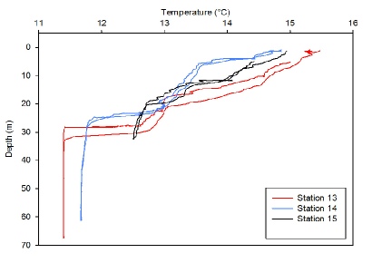
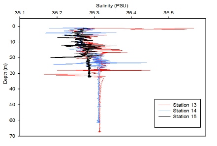
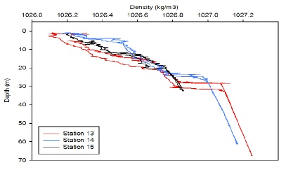
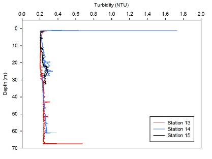
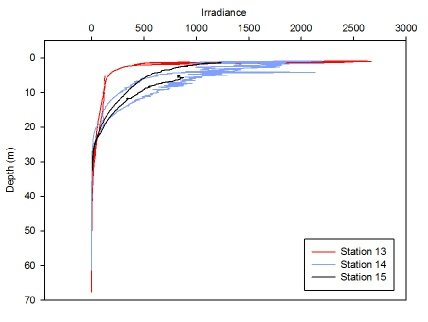
Figure 1- Temperature (°C ) depth (m) profile for all three stations sampled. Taken with CTD.

Figure 2- Salinity (PSU) depth (m) profile for all three stations sampled. Taken with CTD.

Figure 3- Density (kg/m3) depth (m) profile for all three stations sampled. Taken with CTD.

Figure 4- Turbidity (NTU) depth (m) profile for all three stations sampled. Taken with CTD.

Figure 5- Irradiance depth (m) profile for all three stations sampled. Taken with CTD.

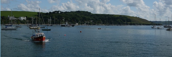
On Wednesday 24th June 2015, Group 9 took part in a scientific research trip on RV Callista to locations off the coast of Falmouth, UK. The trip sampled three depth profiles and net catches, at Stations 13, 14 and 15. It took approximately 5 hours between 07:00 UTC and 12:00 UTC. The first station was the furthest offshore with the subsequent stations successively inshore. Conditions were ideal for sampling with minimal swell and waves, and clear skies with very light winds. The only noticeable wave motion came from close passing ships. The only issue was failure of the plankton net closing at the correct depth.

Low tide 04:19 UTC

High tide 10:08 UTC

Surveying occurred on a neap tide.

Figures 6, 7, and 8 show how the Richardson’s numbers change with depth at each of the stations. The 2 dashed lines on each graph show the boundaries between the turbulent flow (<0.25), laminar (>1). At all 3 stations there have mostly turbulent flow with a few points in each representing laminar flow however there doesn’t seem to be any patterns present as there are points of high Ri values across various depths and temperatures, this is most noticeable at Station 14.

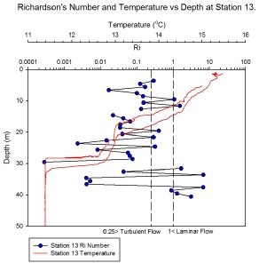
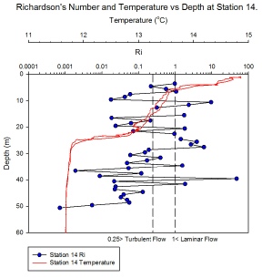
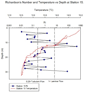
Figure 6- Richardson’s Number and Temperature vs Depth at Station 13. Data taken from ADCP.

Figure 7- Richardson’s Number and Temperature vs Depth at Station 14. Data taken from ADCP.

Figure 8- Richardson’s Number and Temperature vs Depth at Station 15. Data taken from ADCP.

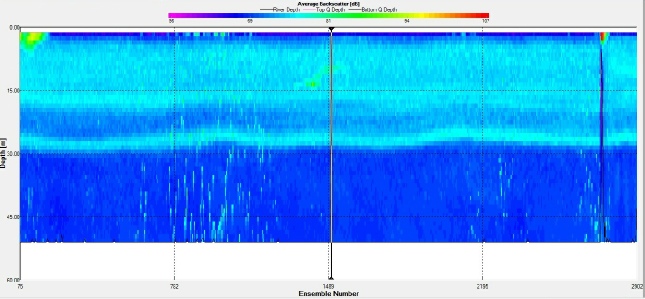
At Station 13 the average backscatter shows us the location of the zooplankton. This conforms to the double thermocline structure observed at this station as well with the below lighter blue structure being within the recorded deep chlorophyll maximum.

Fiedler P.C., 2010, ‘Comparison of objective descriptions of the thermocline’ Limnology and Oceanography: methods, Vol. 8, pp 313-325

Horne E. P. W. and Toole J. M. 1980, ‘Sensor Response Mismatches and Lag Correction Techniques for Temperature-Salinity Profilers,’ Journal of Physical Oceanography, Vol.10, pp 1122-1130

Figure 9 - A graph showing the average backscatter from the ADCP

Table 1 - A table showing the general metadata from Callista