Disclaimer: the views and opinions expressed are those of Group 9 members and not necessarily those of the University of Southampton, National Oceanography Centre or Falmouth Marine School

To attain the data, four pieces of equipment were deployed, a CTD rosette with niskin bottles, an ADCP, a plankton net, and a secchi disk.

Most of the information on the physical properties of the water column would be collected using the CTD which was attached to the rosette with niskin bottles.

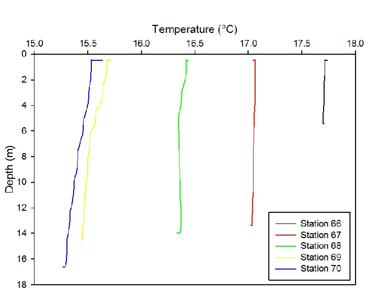
Temperature (Fig 1);- Figure 1 shows a graph of temperature relative to depth for stations 1-5 located down the Fal estuary. The maximum temperature recorded (17.737oc) was recorded at station 66 (0.495m) and minimum temperature (15.257oc) recorded at Station 70 (16.636m). Figure (1) shows that not only does temperature decrease with depth but decreases with distance from the source of the estuary. Stations 68, 69 and 70 show indication of a developing thermocline around 2-4m.  There is no significant temperature change within the temperature profile from Stations 66 and 67. Values plateau at initial and greatest depth within each profile due to deployment and recovery of the CTD.

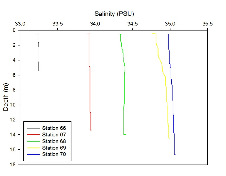
Salinity (Fig 2);- At all 5 stations, the observed salinity was very constant with depth: indicating very strong tidal mixing. This has most likely been exaggerated by the recent spring tide, and the fact the tide was falling for most of the time spent sampling. As expected, the lowest salinity was observed at the top of the river, with salinity increasing on approaching the estuary’s mouth.

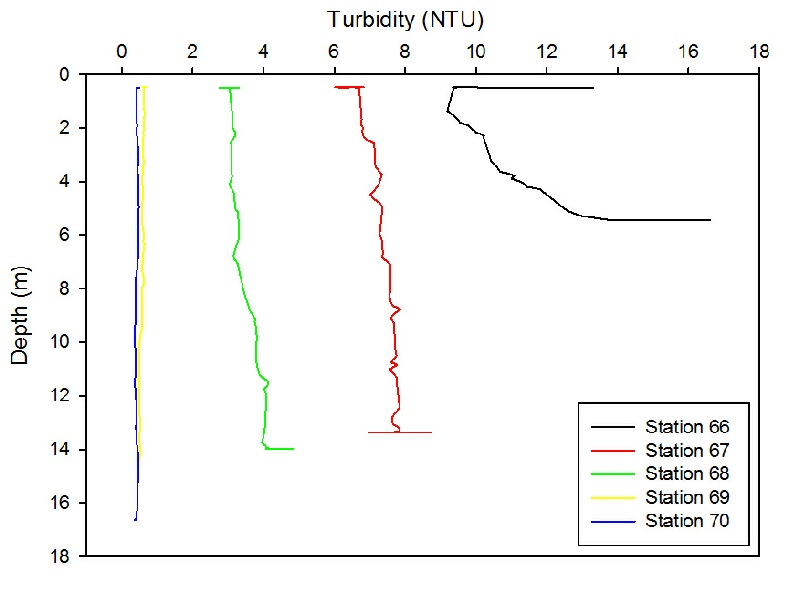
Turbidity (Fig 4);- Turbidity was greatest at the Station 66 (the shallowest station). Surface turbidity at this station got up to 14, decreasing with depth but with a sudden increase at the river bed. The sudden spike could be attributed to the effect of the Bill Conway’s propellers suspending sediment. The surface spike is more unusual and harder to interpret, but again could be a result of propeller wash or a drifting patch of weed (many were observed floating on the river)

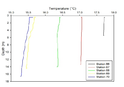
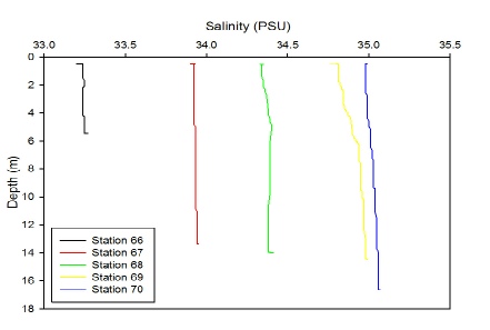
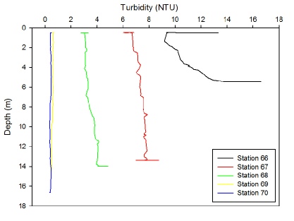
Figure 1- Temperature (°C ) depth (m) profile for all five stations sampled. Taken with CTD.

Figure 2- Salinity (PSU) depth (m) profile for all five stations sampled. Taken with CTD.

Figure 4- Turbidity (NTU) depth (m) profile for all five stations sampled. Taken with CTD.

Aim;- The aim of the research trip was to ascertain the differences between the upper and lower estuary

The physical aim was to create a horizontal transect from one bank to another at each station using an ADCP and to compare the characteristic of different tidal flows.

Method;- The flow of water within the estuary was determined using an ADCP. Facing seaward, the left bank is the bank located on the left hand side, relative to the seaward orientation. Once the boat was positioned at one side of the bank, facing the opposite bank, the ACDP began to log flow measurements. Travelling between 2 and 4 knots, the transect was completed when the boat reached the shallow waters on the opposite bank. ACDP transect images were then saved for further analysis.

Table 1 - A table showing the general metadata from Bill Conway

Figures 5-9 show how the Richardson’s numbers change with depth at each of the stations. The 2 dashed lines on each graph show the boundaries between the turbulent flow (<0.25), laminar (>1).

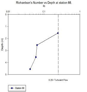
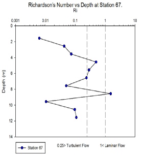
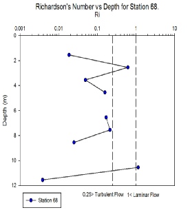
Figure 5- Richardson’s Number vs Depth at Station 66. Data taken from ADCP.

Figure 6- Richardson’s Number vs Depth at Station 67. Data taken from ADCP.

Figure 7- Richardson’s Number vs Depth at Station 68. Data taken from ADCP.

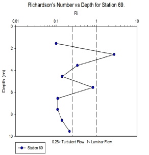
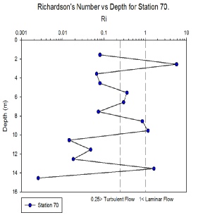
Figure 8- Richardson’s Number vs Depth at Station 69. Data taken from ADCP.

Figure 9- Richardson’s Number vs Depth at Station 70. Data taken from ADCP.

Banner F.T., Collins M.B., and Massie K.S., 1980, ‘The North-West European Shelf Seas: the Sea Bed and the Sea in Motion II. Physical and Chemical Oceanography, and Physical Resources,’ Elsevier Scientific publishing Company, Amsterdam, The Netherlands.

The 5 graphs above (Fig 5-9) show how the turbidity of the water column changes with depth at each of the 5 stations on the estuary. Each of the graphs show that most of the points at each station have a low Richardson’s number indicating turbulent flow throughout the column. However, laminar flow is present on figures 6,7,9  for at least one point. This suggests that the water throughout the estuary are turbulent. Figure 5, which shows the Richardson’s number against depth at Station 66, shows a decrease in Richardson’s number with increasing depth from 0.25 (for boundary for turbulent flow) to 0.04 meaning the water had become more turbulent in this shallow water body as we approached the bottom. This may be due the interaction between the bottom and the water (Banner et al 1980). This would explain the low secchi number as the turbulent flow in a shallow system would re-suspended some of the sediment.

At Station 67 the majority of the column shows turbulent flow apart from at 8.55m where laminar flow is present, a Ri value of 1.53, the surface on the other hand has a very low Ri number of 0.006. The low Ri at the surface at the surface may possibly be due to the rain present at that time causing some turbulence in the surface layer. The high Ri at 8.55m may be the depth between the areas of interaction and mixing between the water and the surface and the water with the bottom. Figure 7 shows that the Ri numbers of the water at Station 68, like 67, is mostly a turbid station but there are some areas of laminar flow at 10.55m with 1.15. At the last 2 Stations (69 and 70), the data is only representative of the top 10-15m instead of the whole column, regardless we can still make inferences about the column with the data present. Like before these two stations are also turbid showing there is mixing present in these surface sections. Station 69, unlike Station 70, appears to have an increasing Ri with depth where it decreases at Station 70.

The total flux of water was measured on each transect at the adjacent station. At Station 66 whist recording data from the CTD we observed a drop in the level of water of 49cm over the 30 minute sampling time with a rate of change of 95cm per hour. Between Stations 67-68 and 68-69 there was a very fast rate of change of 242 and 163cm per hour respectively observed. Between Station 69 and 70 a 61cm per hour drop rate was observed. The reasons for this fast rate of change is down to transect were recorded on an outgoing tide a 3-4 hours before low water where typically the fastest flow rates are observed.

The flushing time of the estuary was calculated from the tidal prism method. It was calculated from rough measurements of the estuary using tools such as google earth as well as charts to determine the average depth of the estuary. This estimated the flushing time of the estuary to be 41.4 hours.

The tidal flushing assumes that a tidal prism of water is removed every tidal cycle this is not the case as water may become entrapped in embayments and other topographical features. therefore we have underestimated the value for the flushing time

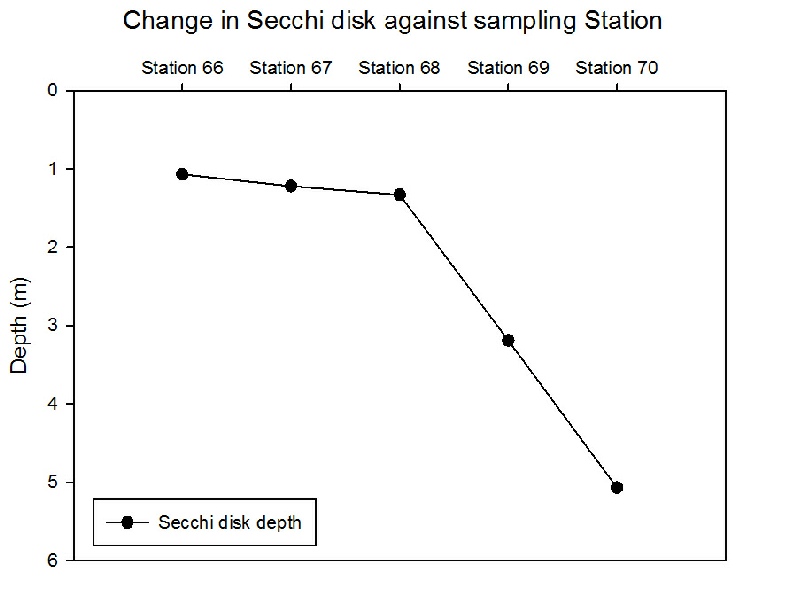
Figure 10 - A graph showing the change in Secchi disk depth