CTD Temperature and Salinity Depth Profiles

A) Station 1

B) Station 2

C) Station 3

D) Station 4

E) Station 5

F) Station 6

G) Station 7

Figures 1A-G illustrate Temperature and Salinity Depth Profiles of all 7 stations along the transect of the Fal Estuary and subsequent river. Data taken on the 27/06/2014 between 07:20 and 12:22 UTC.

(Click individual graphs to enlarge).

ADCP

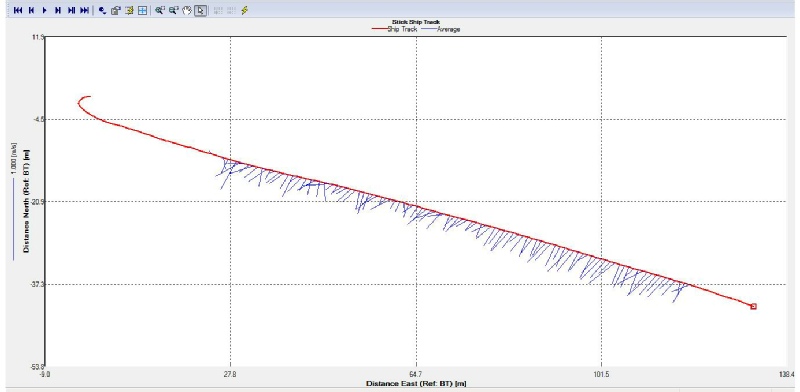
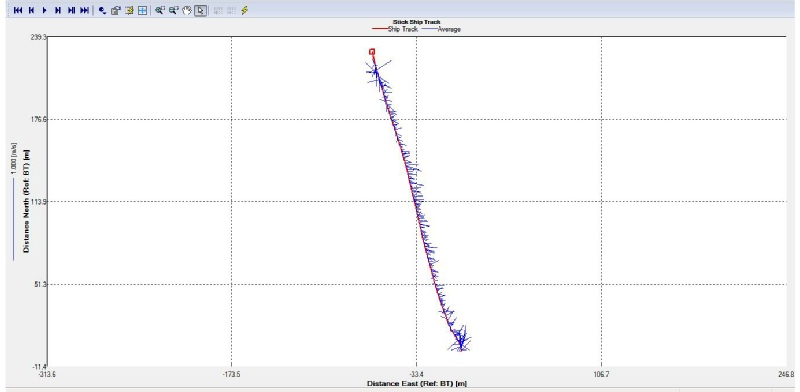
A) Station 1 ship track

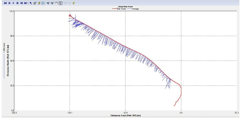
B) Station 2 ship track

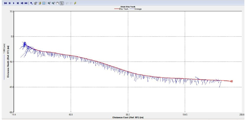
C) Station 3 ship track

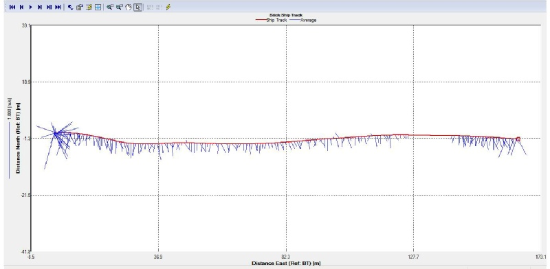
D) Station 4 ship track

E) Station 5 ship track

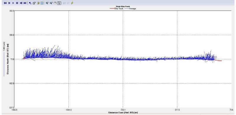
F) Station 6 ship track

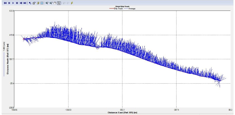
G) Station 7 ship track

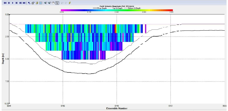
A) Station 1 velocity contour

B) Station 2 velocity contour

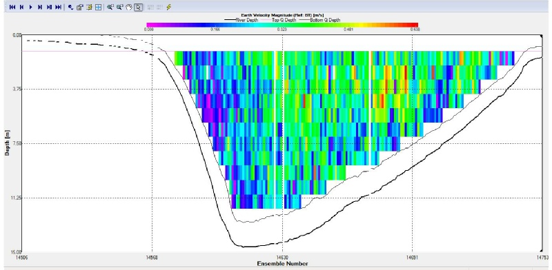
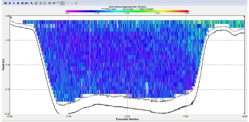
C) Station 3 velocity contour

Figures 2 A-G Illustrate the ship track from the transect line completed at all stations along the Fal Estuary and subsequent river. Data taken on the 27/06/2014 between 07:20 and 12:22 UTC.

(Click individual graphs to enlarge).

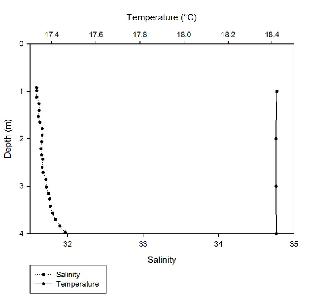
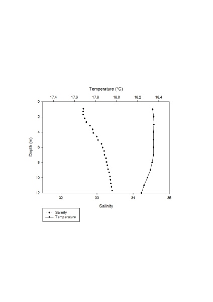
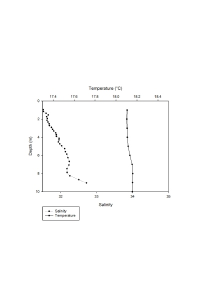
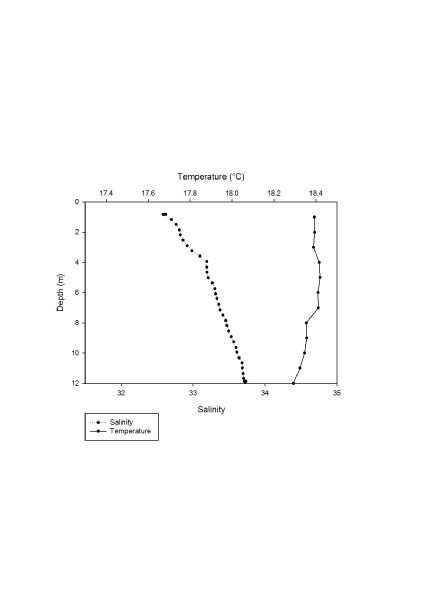
Figure 1A shows that the temperature was constant at 18.4°C within the water column between 1 and 4m. Salinity increased with depth, starting at roughly 31 salinity at 1m depth and ending at 4m depth at a salinity of 32.  Figure 1B shows that the temperature was constant at 18.1°C between 1-4m, it then increased to around 18.2°C from 7-10m depth. The salinity increased with depth from 31 salinity at 1m to around 32.7 at 9m depth.

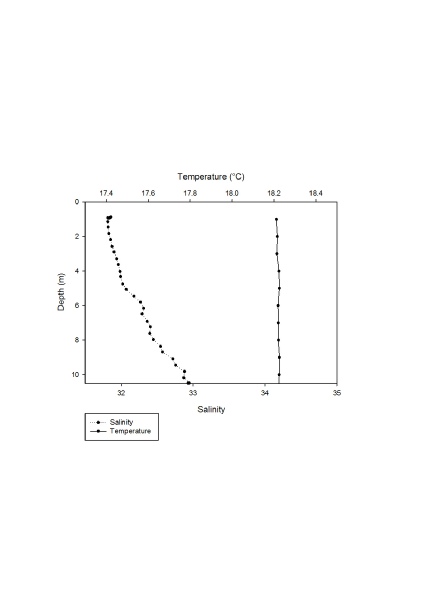
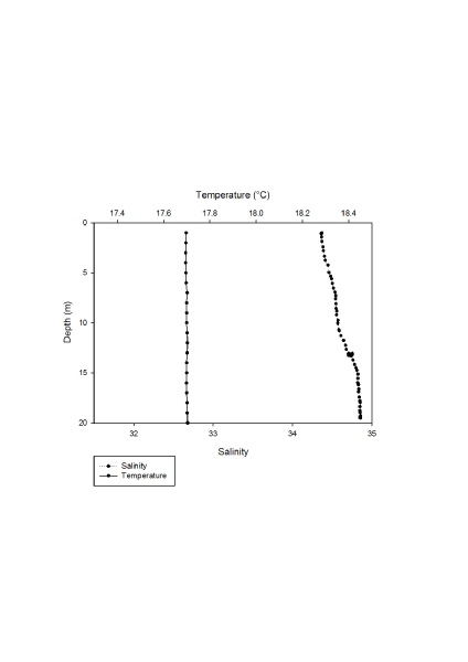
Figure 1C shows that the temperature was constant at around 18.2°C between 1-10m. The salinity decreased with depth from just below 32 salinity at 1m and ending at 33 salinity at 10m. Figure 4 1d for station 4 shows that the temperature remains constant at around 18.3°C between 1-7m and then decreases to 18.2°C at 12m. The salinity decreased from roughly 32.5 salinity at 1m to roughly 33.5 salinity at 12m depth.

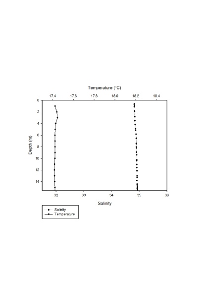
Figure 5 1E shows that the temperature remained constant from 1-3m at 18.4°C, it then increased to just over 18.4°C between 4-7m depth and then decreased to roughly 18.3°C at 12m depth. The salinity decreased between roughly 32.5 at 1m to roughly 33.7 at 12m depth.

Figure 6 1F shows that the temperature remained constant between 1-20m at 17.7°C. The salinity decreased with depth from roughly 34.5 at 1m to just below 35 at around 19m depth.

Figure 7 1G shows that the temperature increased slightly to around 17.3°C between 0-3m and then remained constant between 4m to roughly 16m at just over 17.4°C. The salinity increased slightly between 1m to roughly 16m.

Figure 2A shows that the estuary channel is orientated south-south-westerly and the net flow was shown to also be in this direction across the transect. Flow is found to be <0.5m/s. Figure 2B suggests the estuary channel is orientated to the west-south-west and the transect was situated immediately following a confluence on a meander. The net flow broadly follows the channel, but was orientated more southerly. The flow is shown to be slower on the eastern side of the transect with net flow for the whole transect ~0.5m/s.

At transect 3 (figure 2C) the estuary channel is orientated to the south and the transect was immediately following a confluence of 2 additional rivers to the major estuarine channel. The net flow follows the orientation of the channel to the south with a flow of <0.5m/s, ~0.3m/s.  Figure 2D shows that the estuary channel is orientated to the south and the net flow was also to the south at ~0.25m/s. The most western part of the transect showed some confusion of the flow perhaps showing a corruption of the natural flow by the vessel. There was also a section of bad returns to the east that have been omitted.

Figure 2E implies the estuary channel is orientated westerly at this point and is situated on a large confluence. The flow at this point was shown to be going upstream to the east at ~0.2m/s. This shows the tidal influence at this stage of the cycle.At transect 6 (figure 2f) the estuary channel is orientated to the south and the flow is going upstream to the north, showing a tidal influence. The flow was strongest on the western side of the transect at ~0.5m/s and above, whereas the central channel had a lower flow at <0.2m/s. The eastern side of the transect also showed a slightly higher flow, but not to the same extent as the western side.

Figure 2G shows the estuary channel is orientated to the south and this is the mouth of the estuary. The net flow was variable across the transect and was going upstream due to tidal influence. The highest flow was around 0.8m/s, however the majority was shown to be around 0.4m/s. The flow was fastest in the central and western parts of the transect and the far eastern and western points were less consistent in flow speed and direction. There was also a region towards the centre of the transect where flow was much slower than the immediately surrounding water and was heading downstream.

D) Station 4 velocity

contour

E) Station 5 velocity

contour

F) Station 6 velocity contour

G) Station 7 velocity

contour

Figures 3 A-G Illustrate the velocity contour from the transect line completed at all stations along the Fal Estuary and subsequent river. Data taken on the 27/06/2014 between 07:20 and 12:22 UTC.

(Click individual graphs to enlarge).

Richardson’s Number

A) Station 1

B) Station 2

C) Station 3

D) Station 4

E) Station 5

F) Station 6

G) Station 7

Figures 4 A-G illustrate calculated Richardson’s number against depth for each of the 7 stations along the Fal Estuary and subsequent river. Data taken on the 27/06/2014 between 07:20 and 12:22 UTC.

(Click individual graphs to enlarge).

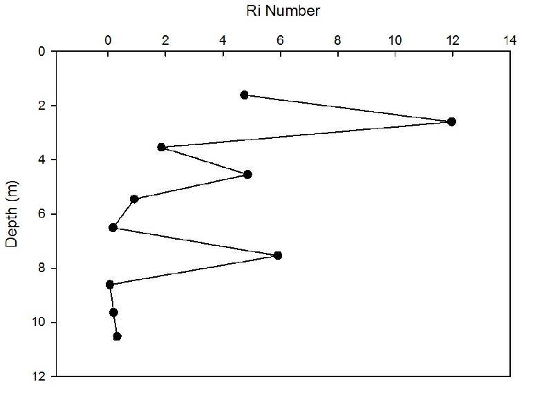
Figure 3A suggests a faster flow on the eastern side of the channel at ~0.3m/s which decreased to the west and with depth down to minimums of ~0.05m/s. The maximum depth was found to be at around 6m and the maximum sampling depth at around 5m.

Figure 3B showed a faster current in the central channel with lower velocities closer to the bed and most significantly on the south-east side. Minimum velocities were seen on the south-eastern bank at ~0.01m/s and maximum velocities in the north-western central channel at ~0.6m/s. Most of the profile shows velocities around 0.5m/s. Maximum depth was ~14m and maximum sampled depth ~12m.

Figure 3C implies faster flow speeds were seen closer to the surface in the central channel at ~0.4m/s. Minimum flow speeds are seen closer to the bed and banks with the lowest velocities being ~0.05m/s. The maximum depth of channel appears to be ~14m and the maximum sampled depth is ~12m.

In figure 3D maximum flow speeds were found in the surface ~3.5m at ~0.35m/s. Flow speeds decreased to a fairly uniform level after 4m depth to ~0.05-0.15m/s. Maximum depth was shown to be ~14m and maximum sampled depth of ~12m. There was a large section of bad returns in the eastern part of the channel on the right.

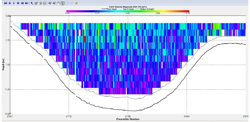
Figure 3E suggests that much of the water at this point was flowing at 0.15±0.1m/s, with the fastest water found in the deep central channel at ~10m depth. The water above was moving more slowly, suggesting different water mass properties with depth and stratification. Maximum depth is shown to be ~14m and maximum sampled depth ~12m.

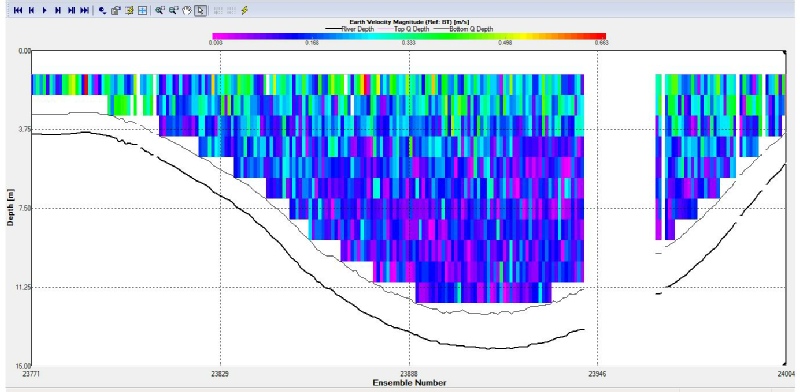
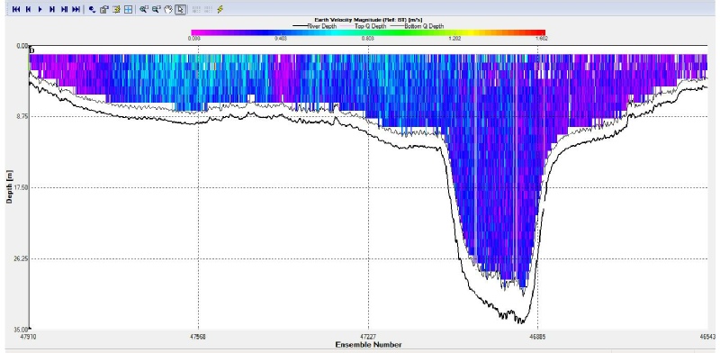
As can be seen in figure 3F, the majority flow speed at transect 6 is around 0.16±0.1m/s with faster velocities in the shallow western side on the right. Flow speed appears to be broadly uniform throughout the water column. Maximum depth was shown at ~25m and maximum sampled depth at ~22m.

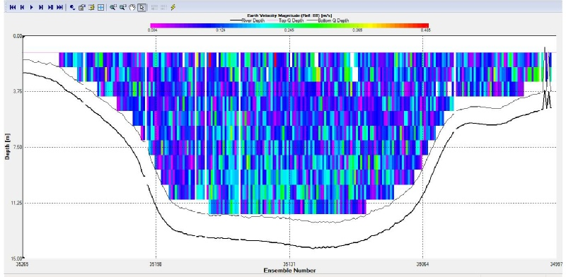
At transect 7 (figure 3G) flow was clearly not consistent across the transect, as on the far banks and in a section to the west of the centre of the channel there were areas of low flow from 0.003-0.2m/s. The central slow flow area had areas of much higher flow on either side, with the highest to the west at ~0.8m/s to the bed and decreasing velocity to the east from ~0.6m/s. A deep channel with a maximum depth of ~34m can be seen in the central east of the channel with flow speeds of ~0.4m/s. Outside of the trench the maximum depth was ~9m and maximum sampled depth of ~8m.

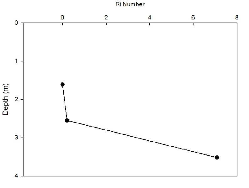
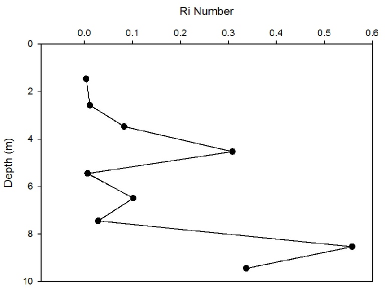
For station 1 (Figure A), the flow is laminar between 1.5m and 2.5m and becomes turbulent between 2.5 and 3m depths.

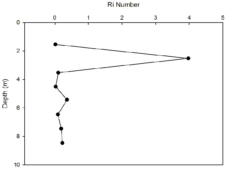
At station 2 (figure B), the Ri first increases rapidly between 2m and 3m depth to an Ri of 4, indicating turbulent flow. Flow then remains constant at Ri of 0 between 4m and 9m, indicating laminar flow.

For station 3 (figure C), the majority of the water column has a laminar flow, with turbulent flow found at around 4m and 8-9m depth, with Ri at 0.3 and 0.55 respectively.

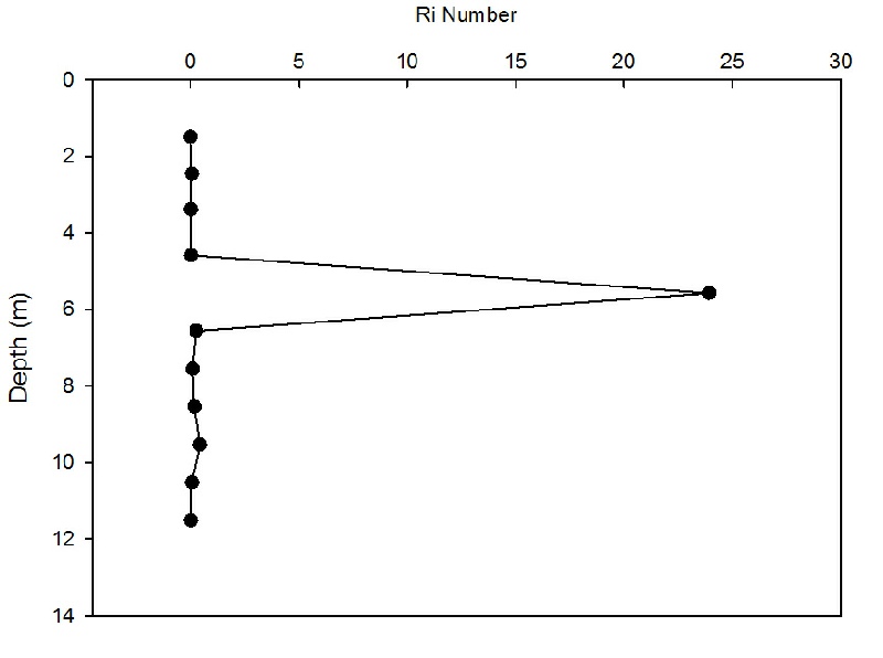
At station 4 (figure D),the Ri remains constant with a laminar flow at 0 between the surface and 12m, with the exception of a rapid increase in the Ri to 25 at roughly 6m depth, indicating turbulent flow.

At station 5 (figure E), the flow appears to be turbulent between the surface and 5m and mostly laminar between 5m and 11m, with the exception of turbulent flow at 8m.  

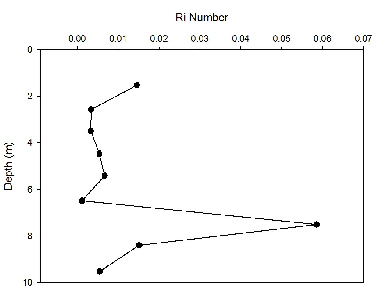
At station 6 (figure F), the flow remains laminar throughout the entirety of the water column sampled, with Ri between 0 and 0.01. There was an increase in Ri to 0.06 at 7m depth.

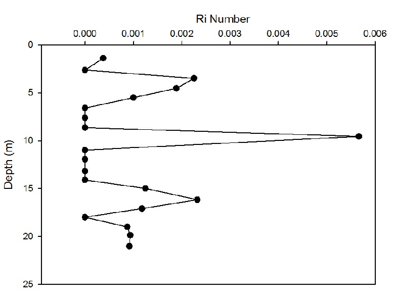
At station 7 (figure G), there is fluctuation in the Ri with depth, ranging from 0 to 0.002; the flow was laminar throughout the water column. At 10m, there was a large increase in the Ri to roughly 0.0057.

Secchi Disk

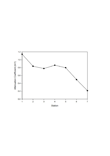
Figure 5 illustrates the attenuation coefficient for all 7 stations along the Fal Estuary and subsequent river. Data taken on the 27/06/2014 between 07:20 and 12:22 UTC.

(Click individual graphs to enlarge).

Figure 5 shows that there was an overall decrease in the attenuation coefficient for the secchi disk depth from station 1 to 7. Station 1, near the river end, had the highest attenuation coefficient of around 1.2 m/1. Station 7, near the marine end, had the lowest attenuation coefficient of around 0.2 m/1.

The further along the estuary you go the smaller the attenuation coefficient and the further light penetrates. This could be because at the river end of the estuary there is more suspended sediment.

Disclaimer - These views are of the students of group 11 only and do not reflect the views and opinions of the National Oceanography Centre or the University of Southampton.