

University of Southampton 2015©


PHYSICAL ANALYSIS

GO TO:

The temperature-depth profile in Figures 1-2 clearly shows the position of the seasonal thermocline (around 27m depth) and the thermal structure of the water column. Below 27m, the temperature of the water is constant showing that there is no influence of mixing from the surface layers. Seasonal thermoclines occur when average wind stress on the surface waters is lower during the spring and summer months. The decrease in winds at this time decrease the depth to which the water can be mixed, creating a shallow layer of warmer water situated on top of a well-mixed cooler layer. The seasonal thermocline then concentrates the phytoplankton into the surface waters, as seen in the Offshore Chlorophyll section. Since the data from stations 35-39 (Figure 2) show the same trends as was collected at station 40-44 (Figure 2 ), it can be assumed that the thermocline is not daily, but perhaps seasonal instead.
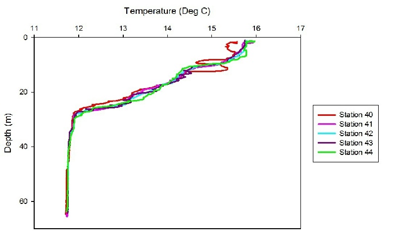

Figure 1 - Depth profile for temperature at each time series station (35-39) - morning
(Click to expand)


The salinity profile from the CTD (see Figure 3) is challenging to interpret due to the salinity spikes occurring up to a depth of 25m. The salinity spikes are caused by an equipment error; a delay in response between the temperature and conductivity sensor. If averaged, there is a constant average salinity of around 35.3. At the very surface, there is notably higher salinity (up to 35.8). It is possible that this is due to surface evaporation creating a shallow layer of high salinity water.
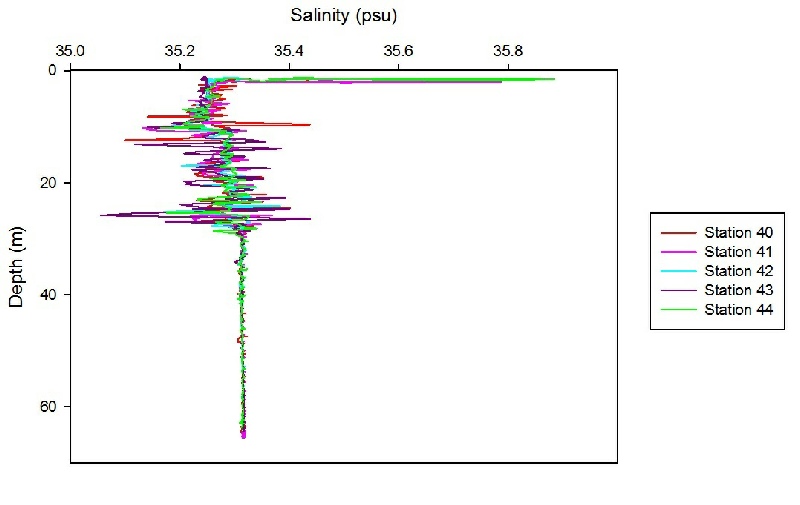

Figure 3 - Depth profile for salinity at each time series station (40-44) - afternoon
(Click to expand)
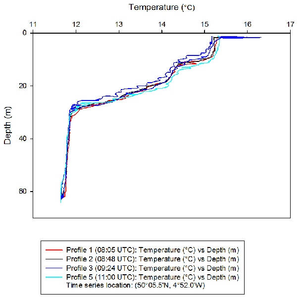

Figure 2 - Depth profile for temperature at each time series station (40-44) - afternoon
(Click to expand)

RESULTS:
RESULTS:

RESULTS:

The irradiance data in Figures 5-6 shows the exponential dissipation of light energy in seawater. The data remained the same throughout the day.
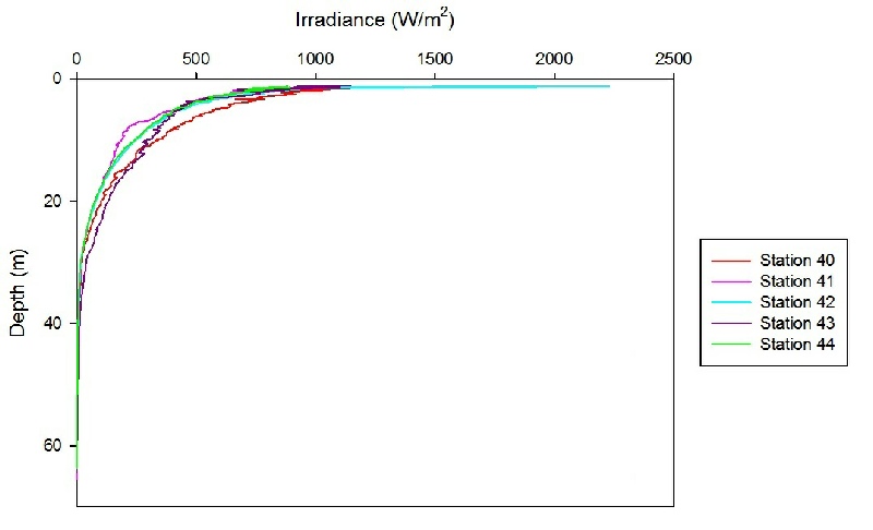
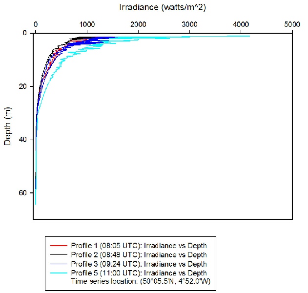
Figure 5- Depth profile for irradiance at each time series station (35-39) - morning
(Click to expand)
Figure 6 - Depth profile for irradiance at each time series station (40-44) - afternoon
(Click to expand)
Current
Mixing

The Richardson number, as discussed in Estuary Physical Analysis - Mixing is a dimensionless number that is used to evaluate the state of the water column with respect the Kelvin-Helmholtz evolution. This determines if the flow is laminar, turbulent or in the transition zone.
Stations 1, 2, 4, and 5 all show a Ri<0.25. This low Ri means that the water column is turbulent and there is a lot of vertical overturn generally. The exception to this pattern is at roughly 5m and 30m where the water column reaches the transition zone; the point that lies in-between laminar and turbulent flow.
Over depth across all stations, despite clear spikes seen towards relatively higher Ri numbers, there is a general trend to a decrease in Ri number. This could possibly be because of more stable conditions below the seasonal thermocline.

RESULTS:
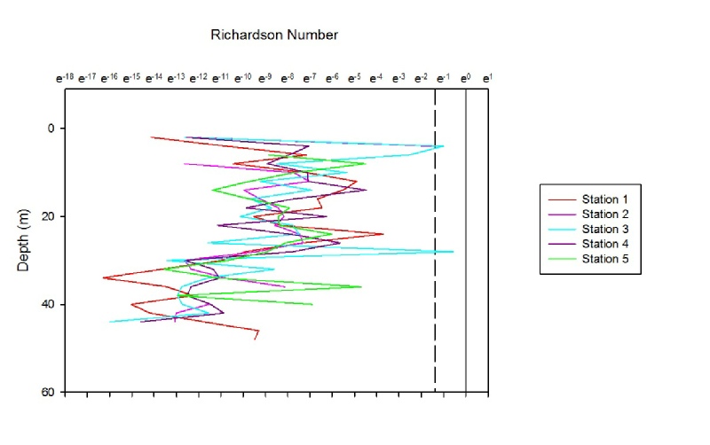

Figure 4 - Depth profile for Richardson Number at each time series station (40-44) - afternoon. Reference lines show boundary between turbulent flow (<0.25) and laminar flow (>1)
(Click to expand)

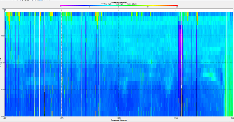
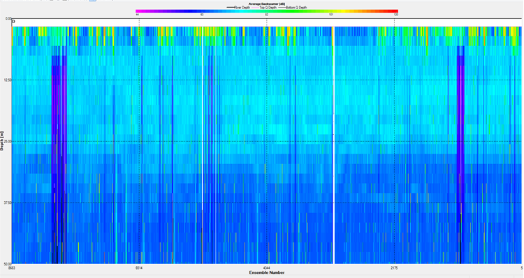
Figures 7-8 - Average backscatter for a) station 35-39 (morning), and b) station 40-44 (afternoon).
(Click to expand)
A)
B)

RESULTS:

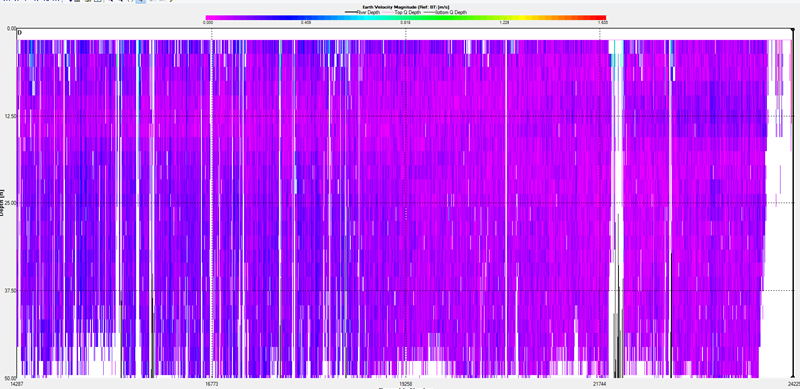
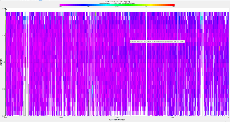
The ADCP data collected shown in Figures 8 & 10 were collected from the same station throughout the day, creating a usable time-series data set. A different group took the first ADCP data set (Figures 7 and 9) while we took the second set of data to complete the time-series. The ADCP figures shown depict the average backscatter (dB).
As you can see from both files, they show similar patterns with regards to the backscatter, with a clear layer seen at around 25m depth. Figure 8 shows a greater amount of backscatter in the upper 5 meters of the water column. There are two areas of distinctively lower backscatter shown by purple that are superseding area of high backscatter at the surface on Figure 8, with a similar pattern seen for Figure 7. These areas are caused by an anomaly on the ADCP, which can be seen by the velocity data on Figures 9 and 10, where no good data can be obtained in the lower backscatter areas of the time-series.
On both backscatter plots, the thermocline can be seen by the clear change in backscatter observed at around 25m depth. Below this point, there is a notable change in overall backscatter, with values around 66dB. In Figure 7, the thermocline is marginally deeper over the series. This could be caused by vertically migrating zooplankton that moving this backscatter layer.

Figures 9-10 - Earth velocity magnitude for a) station 35-39 (morning), and b) station 40-44 (afternoon).
(Click to expand)
A)
B)