

University of Southampton 2015©


PHYSICAL ANALYSIS

GO TO:


Temperature profiles taken in the estuary (Figure 1) show that the water cools slightly the closer it is to the mouth of the estuary; between station 8 and 15, the surface temperature cools by 1.5°. The closer to the opening of the estuary, a thermal structure can start to be observed between 5m and 10m depth.
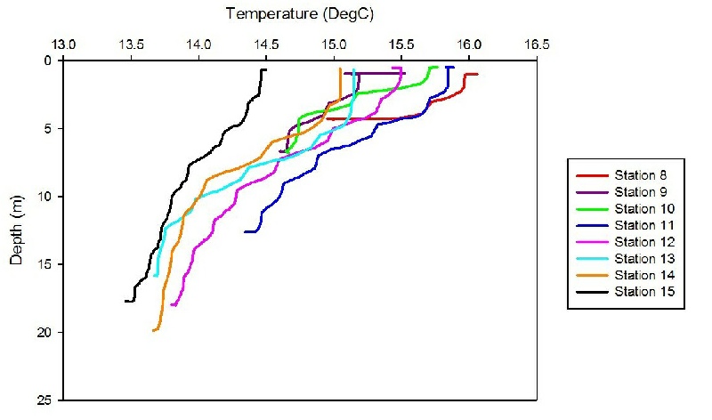

Figure 1 - Depth profile for temperature at each station.
(Click to expand)

Homogeneity in the water column at the various stations in the estuary increases the closer to the mouth of the estuary. This is likely to be due to the direct mixing of the water column by the tide. The change in surface salinity is also affected by the input of freshwater from the Truro and Fal rivers.
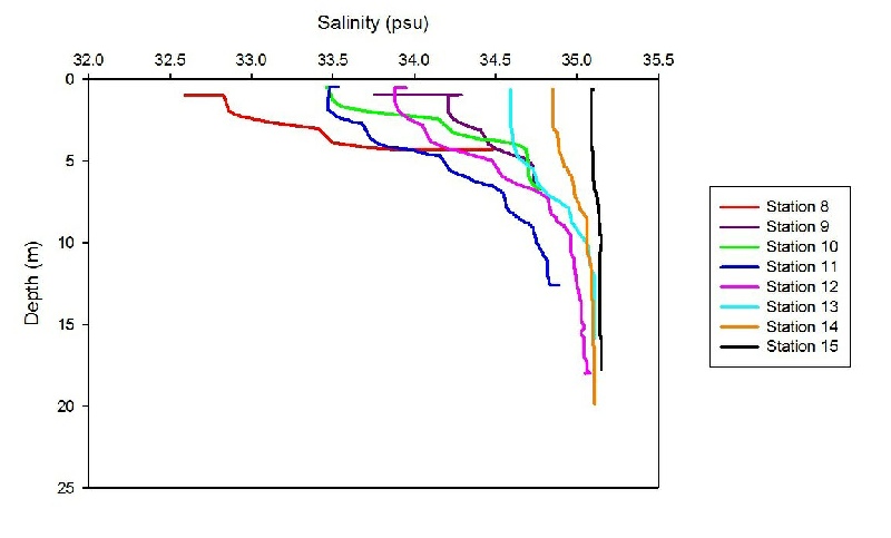

Figure 2 - Depth profile for salinity at each station.
(Click to expand)

RESULTS:

RESULTS:

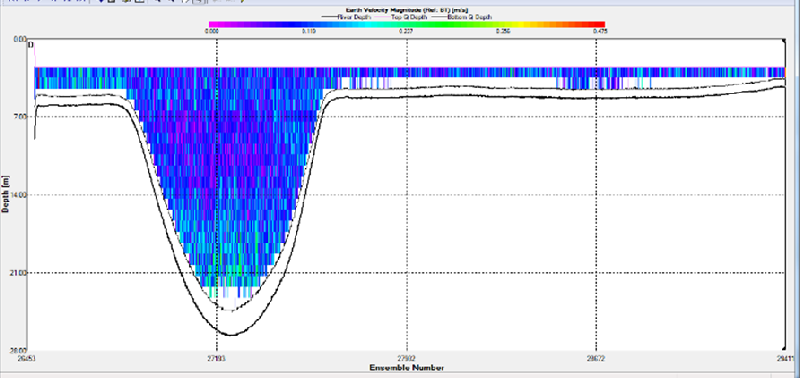
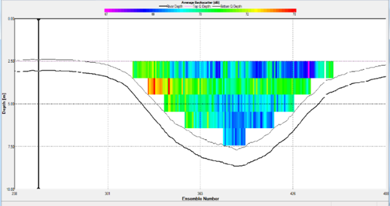
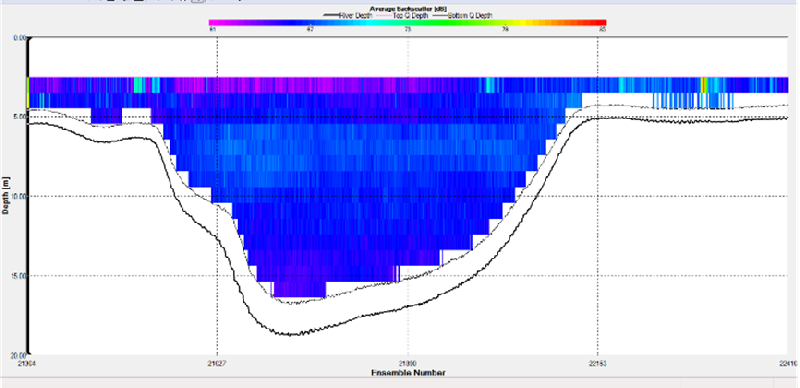
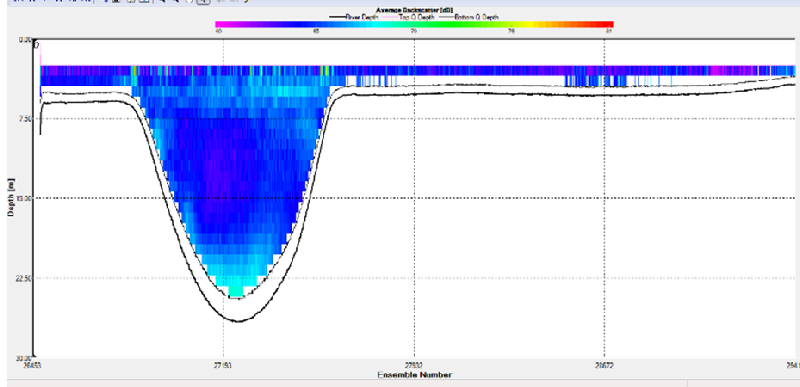
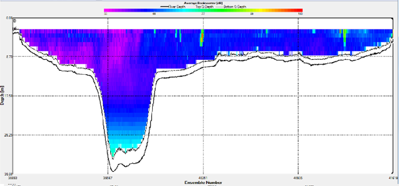
Figure 16 to 22 -Average Backscatter for each station progressively.
(Click to expand)

(See Figures 8 - 22)
As you would expect, there is a change in magnitude and average backscatter throughout the water column downstream of the estuary toward the entrance of the estuary at Blackrock. This is because of a change in friction against the bed/banks downstream as well as a change in biology due to anthropogenic and chemical factors downstream.
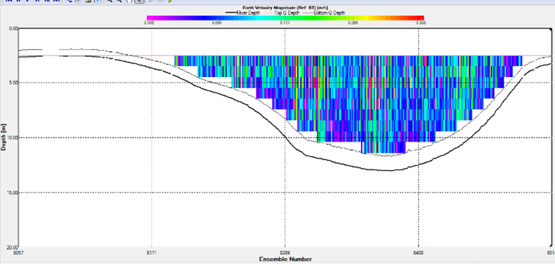
At station 8 you can see a high backscatter from the acoustic signal, particularly on the western bank where average backscatter in dB reaches up to 73. This is suspected to be because of the meandering Truro River as seen in the google image of the stations. The Truro bends round to the right so there will be greatest friction on the estuary bank on the eastern side, creating high turbidity and thus high backscatter. There is a layer of higher backscatter at around 3-4m depth which could possibly be a layer of phytoplankton blooming at the nutricline. The Earth velocity magnitude for station 8 shows the effect of the meandering river on the flow, with a consistent decrease in flow on the eastern side represented by the darker colour on the Winriver data.
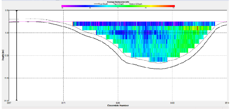
Station 10 (9) shows lower a general lower backscatter value throughout, particularly emphasized at the surface with a layer of low backscatter. There is also an exception with increased backscatter in the eastern bank, again due to the path of the Truro. Magnitude value are fairly consistent throughout.
The backscatter at station 11 is relatively consistent throughout the cross section, with a lower area at the western river bed. This station is deeper than station 8 and 10 (9) so the acoustic signal could be absorbed by the water column/sea bed rather than reflected. Again this station was obtained on a meander of the Truro, contributing to the higher backscatter at the western side of the river bed. Friction The magnitude at this station shows an alternating pattern of higher and then lower velocities in ms-1.
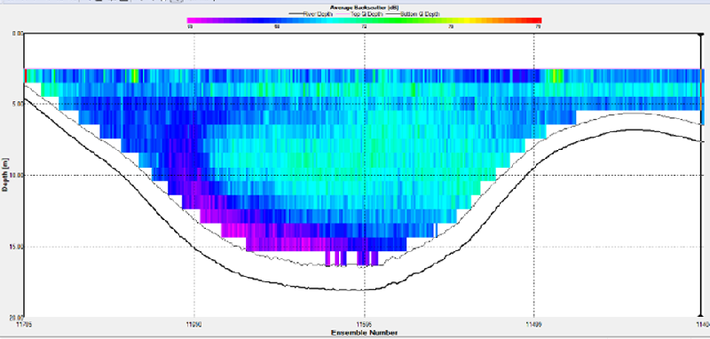
Station 12 shows a very consistent lower backscatter value throughout the water column ranging from 62-72dB apart from a small section in the far western edge reaching up to 99Db. The magnitude data is unusual in that it shows three distinctive areas of current from the surface to depth, with the lowest values on the western edge again, corresponding with the maximum backscatter.
Station 13 was taken at the point where the Truro River enters the Fal estuary. The backscatter shows relatively similar values to station 12 regarding dB. There is one ADCP cell shown that reaches up to 85dB, but this is very small and could have been an error with the ADCP signal. The magnitude shows a stratification in the current with higher values in the upper column. This represent the influence of the river on the estuary, where at this entrance point to the estuary, the river has a large influence on the flow in the estuary.
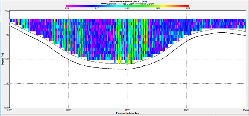
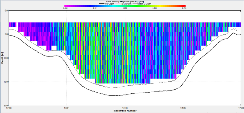
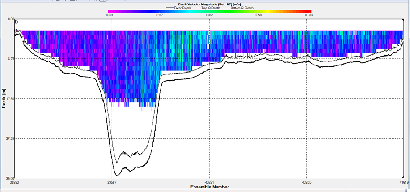
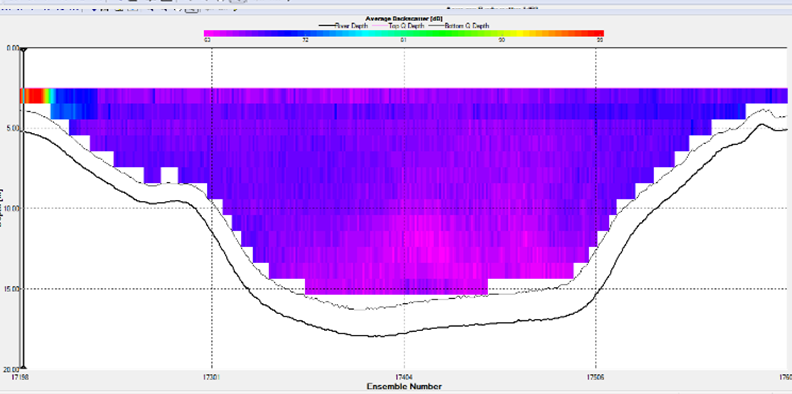
Station 14 was taken in a wide part of the estuary, so had a long ADCP trace. There is a significant increase in depth across the transect reaching down past 22m with the rest of the channel measured around 7 meters. The magnitude throughout the section is consistent, with a lower area of flow observed in the middle of the 22m section. This could be because of the shear between surface river flows and tidal flows creating an area of turbulence and lower velocity flow. The highest level of backscatter is shown to be at the estuary bed in the deep section of the transect.
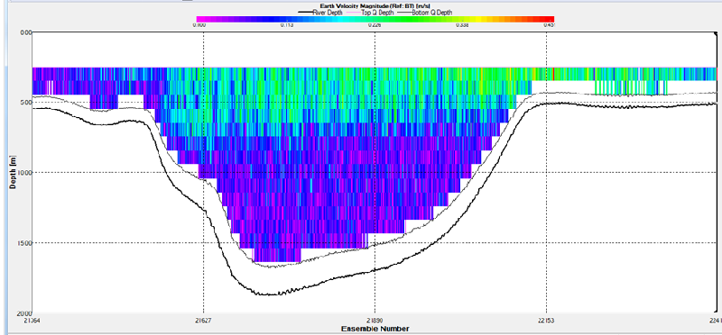
Station 15 was taken at the mouth of the Fal estuary at Blackrock. Here again the water column deepens with again a significant change seen going past 26m. There is a lower backscatter value on the western side. This low section is consistent with the low magnitude value on the western side. The low magnitude of flow could mean sediment falls out of solution, thus a lower constituent value.

References:
[1] Centre for Ecology & Hydrology [Online] Available: http://www.ceh.ac.uk/ [Accessed: 2015, July 1st] (2015)
[2] Ketchum, B. H., Rawn, A. M. The flushing of tidal estuaries. Sewage and Industrial Wastes, 23(2), pp 198–209. (1951)

The Richardson number is a dimensionless number used to measure the vertical mixing in the water column, by evaluating the turbulent state of the water. If the Ri<0.25 then the flow is said to be turbulent, thus leading to vertical mixing. If the Ri>1 then the water column is said to be laminar, and thus a stratified water column.
As you can see from stations 8-14 on Figure 5, despite the large variation in the Ri number, all stations lie below 0.25 which means that the water column is turbulent, and therefore vertically mixed. Only two Ri numbers could be collected for station 1, so this could be the reason that station 1 does not fit with the general trend of stations 9-14.
Station 15 was taken at Blackrock; the mouth of the estuary. There is a spike of Ri at around 15m depth, stretching Ri>1.This means that, at 15m depth, the water column changes to laminar flow. But due to the pattern of station 15 at other depths, and other stations not showing any similar trend, anomalous data for this point can be assumed, and the water column remains turbulent at all depths.
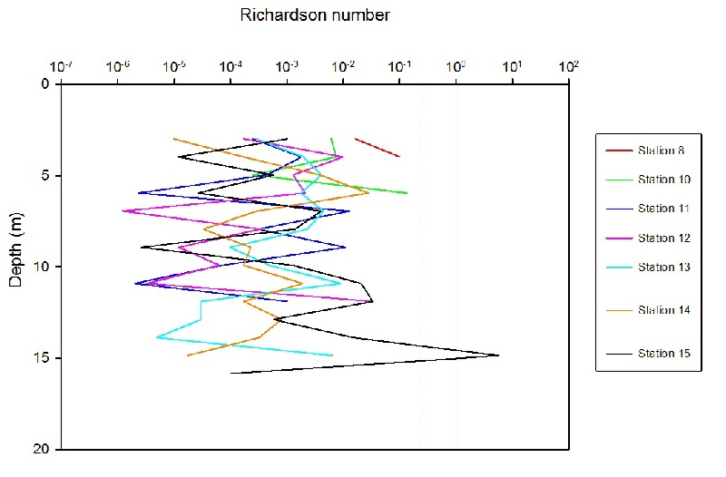

Figure 5 - Depth profile for Richardson number at each station. Reference lines show boundary between turbulent flow (<0.25) and laminar flow (>1)(Click to expand)

The turbidity decreases as the stations reach the mouth of the estuary (Figure 4). The rivers contain suspended material and carry this material into the estuary creating high turbidity at stations within the main channel of the river (stations 8-11). The further the water flows towards the sea, the river flow is opposed by tidal flow and the suspended material falls outs of suspension and settles out, decreasing the turbidity between station 12-15.
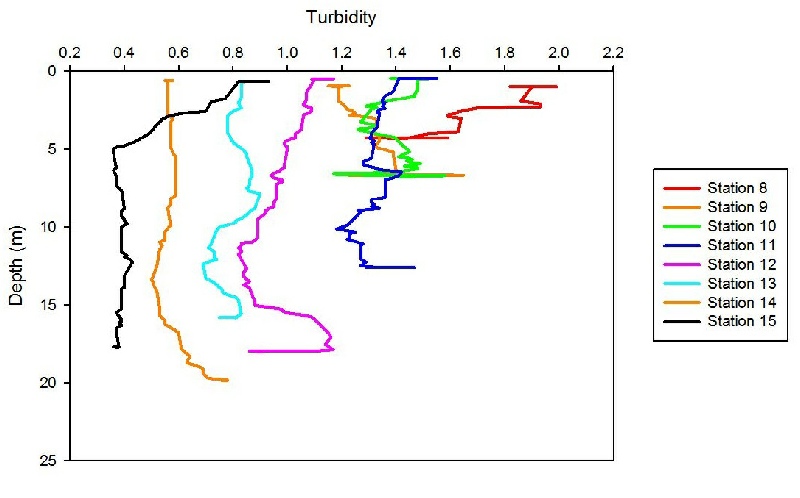
Figure 4 - Depth profile for turbidity at each station.
(Click to expand)

RESULTS:


CALCULATION:
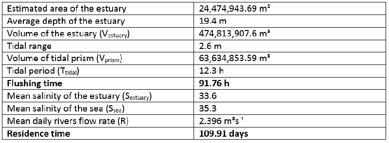
To calculate the flushing and residence times, the following equations were used:
Flushing time = ([Vestuary]/[Vprism]) x Ttidal
Residence time = ((1- ([Sestuary]/[Ssea])/R) x Vestuary
(Where:
Vestuary = the volume of the estuary (m³)
Vprism = the volume of tidal prism (m³)
Ttidal = the tidal period (hours) on the sampling date (24/06/2015)
Sestuary = the mean salinity of the estuary
Ssea = the mean salinity of the sea
R = the river input flow rate (m³s-¹))
The volume of the estuary was calculated by multiplying the mean depth from the 7 stations with the area of the estuary. The area was estimated by drawing an outline using Google Earth Pro. The volume of the tidal prism was calculated by multiplying the estimated area of the estuary with the tidal range on the sampling date. The mean salinity of the sea was calculated using the offshore practical data. The river input flow rate was taken from the Centre for Ecology & Hydrology (rivers Fal and Kenwyn) [1].


Important assumptions when calculating the flushing time using the method of the tidal prism:
(1) The entering water is completely mixed with the water in the estuary at low tide
(2) The volume of water escaping the estuary during the ebb tide does not return during the next flood tide [2]
The calculated residence time of the estuary was 110 days, meaning that it would take a relatively long time for pollutants to leave the water, being

Figure 6 - Flushing and residence time calculations.
(Click to expand)
potentially harmful. The long residence time may be due to the type of the estuary, where the influence of the sea is much greater than the influence of riverine inputs. The calculated flushing time of the estuary describes that it would take 91.76 hours (3.8 days) for the water in the estuary to be replaced with new inputs from the river.
Inaccuracy in the data, such as in the mean depth of the estuary or in the estimation of the area, even when small, can produce a great change in the results.

SAMPLING AND ANALYSIS:
At each station a Secchi disk was lowered into the water, and the depth at which the disk was no longer visible was measured, giving us information on light penetration and turbidity. The euphotic zone (3x the Secchi depth) and the light attenuation coefficient (k value = 1.44/Z, where Z is the Secchi depth) were then calculated.

The graph (Figure 7) tells us that, overall, from stations 1 to 7, the attenuation coefficient decreases, i.e., the closer you get to the English Channel, the further light penetrates the water column. The river end may have had a greater concentration of suspended sediments, explaining the higher attenuation coefficient values in the upper estuary.

Figure 7 - Attenuation coefficient at each station.
(Click to expand)

SAMPLING:
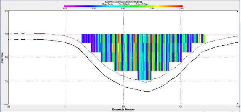
At each station, an ADCP was used to measure current flow and direction throughout the water column, and the data was instantly put into a number of graphs.
Figure 8 to 15 - Earth velocity magnitude for each station progressively.
(Click to expand)

RESULTS:

RESULTS:

RESULTS:

RESULTS:

Estuary type:
It can be determined from the salinity contour plot (Figure 3) that the Fal Estuary is a well-mixed estuary. Salinity remains relatively constant with depth, and decreases as you move further up the estuary. This is due to the strong tidal currents compared to the river flow, causing an even mixing throughout the estuary.
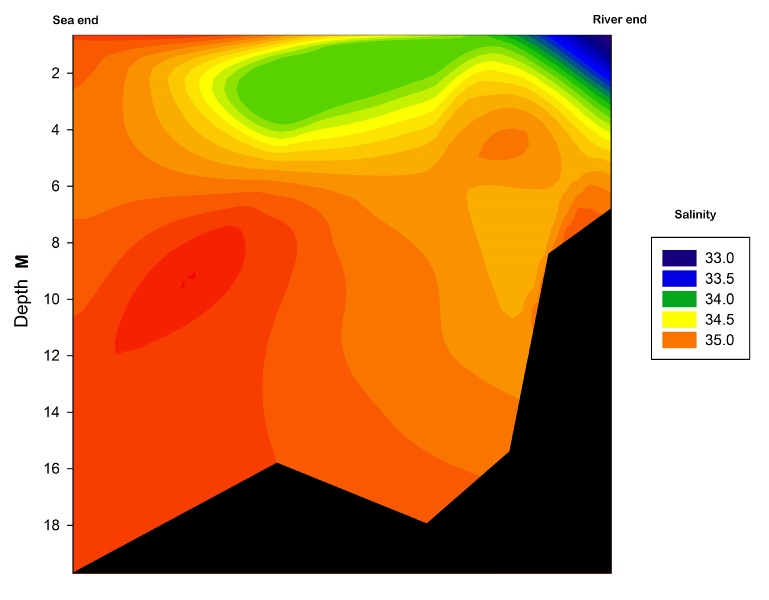

Figure 3 - Salinity contour plot for the estuary.
(Click to expand)