
Disclaimer: These findings are the personal interpretation of the students involved and do not reflect the views of the University of Southampton, the National Oceanography Centre or Falmouth Marine School.


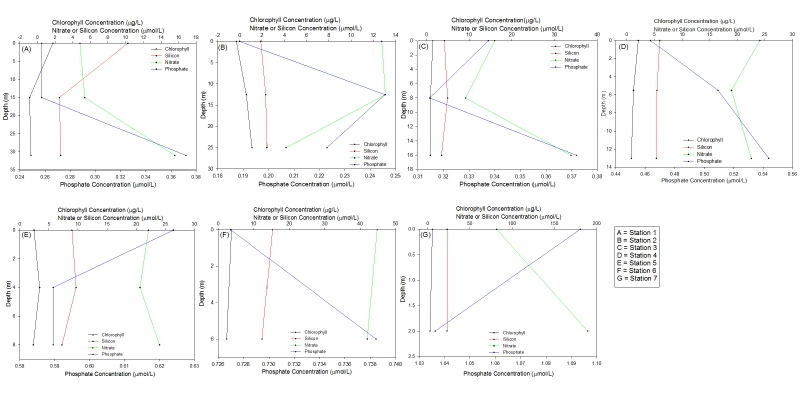
Figure 15
Chlorophyll
Method
The chlorophyll samples collected from the seven stations on the Fal Estuary were frozen overnight instead of using a sonocater. The absorbance was then determined using a 10-au Turner Fluorometer. The negative chlorophyll readings seen in samples from Stations 1 and 2 are considered anomalous results. After Station 2 the method was changed and the samples were shaken before the absorbance reading was taken. The concentration of chlorophyll was calculated using the equation: Concentration = 7/50 x Absorbance.
Interpretation
The chlorophyll concentration, used as an indicator for phytoplankton abundance, increases slightly up the estuary with slightly higher values from Station 7 than Station 1 (fig 15). This could be due to increased nutrient from freshwater inputs, however the data is inconclusive. It could also be due to a reduced amount of flushing higher up the Estuary, as the Stations in the Upper meandering section of the Estuary have slightly higher concentrations of chlorophyll than the lower Estuary which would be more affected by tidal flushing.
The chlorophyll concentrations generally show a slight decrease with depth, as expected, as the phytoplankton will tend to stay in the surface waters due to the increase in light intensity. Station 5 shows an increase of chlorophyll at around 4m (fig 15) suggesting that this is the are with the highest nutrient levels with a light intensity great enough for photosynthesis. This is a trend commonly seen with phytoplankton, with the maximum concentration found at the bottom of the euphotic zone.
Chemistry of the Estuary

Nitrate
Determination of nitrate levels by fluid injection
Firstly, the already filtered bottled samples collected from the estuary on Conway had to be filtered a second time with a syringe and detachable filter. This made sure that all particles are eliminated that might have passed through the primary filtration (undertaken on Conway), as these particles clog up the injection tubes which have a very small diameter on the inside.
The filtered water sample is then injected into the system of tubes and passes through the granules of a copper containing compound, catalysing the reduction of nitrate to nitrite. This is needed as it is nitrite that is used in the cell placed in the spectrometer. The injection of the fluid takes a couple of minutes to reach the cell and then absorbance values are given off via a chart recorder that draws the peaks of each individual sample, with each sample being run through the system twice for greater accuracy.
The length of the peak drawn can be measured and the nitrate levels determined by a calibration plot by recording the peaks of standards made with known nitrate concentrations.
A theoretical dilution line was plotted using the sea end member and a previously collected river end member from the river Allen above the point of saltwater influence. The relevant nitrate concentrations for these end members were plotted against salinity values, likewise, all sampled data was plotted against their corresponding salinity values between 35 and 27 salinity units.
Interpretation
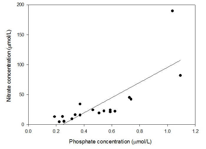
Interpretation of the relevant conservative/non-conservative nature of nitrate (fig 10) is complicated by the limited range of salinity values. It could be that as the majority of data points are below the theoretical dilution line (TDL) the nitrate is acting non-conservatively towards the seaward end of the estuary with nitrate being stripped out of the water column. Likewise, a high concentration (189.28 µmol/L-1) at the lowest measured salinity value (27) may suggest that as salinity decreases towards the river end member, it would produce nitrate levels that would appear above the TDL. This assumption is further complicated by the fact that the high sample was recorded at 2m and a further surface sample at 1m was considerably lower (81.80 µmol/L-1). One might assume that higher nitrate concentrations may be found in the surface water which would have greater freshwater influence which may suggest that the data point is an anomaly. Therefore, when looking at the nutrient/chlorophyll depth profiles (fig 15) it may be suggested that previous stations (E and F) had reasonably uniform nitrate depth profiles whereas, the depth profile of the final sample station G covers a broad range suggesting an error in the sampling method and should therefore be disregarded. However, with only one data point above the TDL, this assumption is purely speculation and requires further data collection towards the river end member before any validation can be made.
Phosphate
Method
The amount of phosphate sampled from the estuary was measured using a spectrophotometer (HITACHI U1800) and the method fromT.R. Parsons et al. (1984) “A manual of chemical and biological methods for seawater analysis”. The data was input into a spreadsheet and the absorbance values corrected. The correlation between the phosphate concentration and blank corrected values was determined using the equation y = 0.0873x + 0.0002 and was an almost perfect fit with an R squared value of 0.9994.
Interpretation
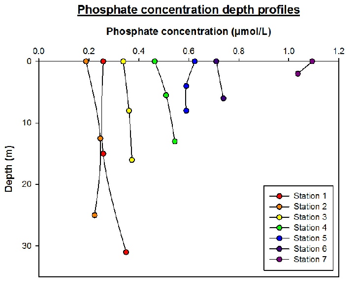
For each station, phosphate had little change with depth, at the most an increase or decrease of about 0.1µmol. The estuarine mixing diagram showed non-conservative behaviour with almost all of the points plotting above the theoretical dilution line, suggesting addition of phosphate (fig 12). Phosphate is often a large component of fertiliser run-off which could explain the high addition of Phosphate throughout the Estuary. The addition could also come from sewage effluent from nearby sewage plants. There is a long residence of 52 days and 2 hours, which will allow a high build up of Phosphate throughout the estuary. As seen in figure 10 Nitrate is removed throughout the estuary, suggesting that this is the limiting nutrient in phytoplankton growth (fig 11), allowing a high build up of Phosphate.
Figure 11
Silicon
Method
In the laboratory, we used a slightly modified Mullin and Riley (Anal Chim Acta 12: 162, 1955) procedure to determine the amount of silicon present in the samples. We mixed the water samples with a solution called Molybdate, which results in the formation of Silicomolybdate, Phosphomolybdate and Arsenomolybdate complexes. A reducing solution consisting of metol sulphate, oxalic acid and sulphuric acid, was then added to the samples. The reducing agent decomposed any phosphomolybdate and arsenomolybdate within the samples, resulting in the silicomolybdate being the solitary complex remaining within the samples. This delivers a blue colour, of which the intensity varies depending on the amount of silicomolybdate present. We then used a spectrometer to measure the absorbancy of the samples. In addition to calculating the amount of silicon present in the samples, we also needed to detect if there was any silicon present in the reagents used, as these would alter our estuarine samples, causing invalid results. To do this we prepared a blank solution using MQ grade water instead of seawater and measured the absorbancy of this as well as the other samples. The results were then corrected to account for the MQ grade water results to ensure they were taken out of our estuarine samples.
Interpretation
It is clear from figure 14 that silicon is acting conservatively throughout the estuary, based on the fact that our silicon plots are in line with the TDL (Theoretical Dilution Line). Nearer the mouth of the estuary, some plots fall below the TDL. This indicates some slight removal of silicon within this area. This could be due to a higher bloom of phytoplankton stripping away some of the nutrients. However this can only be an assumption, as further sampling and observations would be needed in order to prove this.
Figure 13
Figure 12
Figure 14
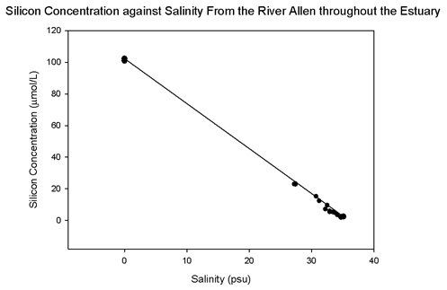
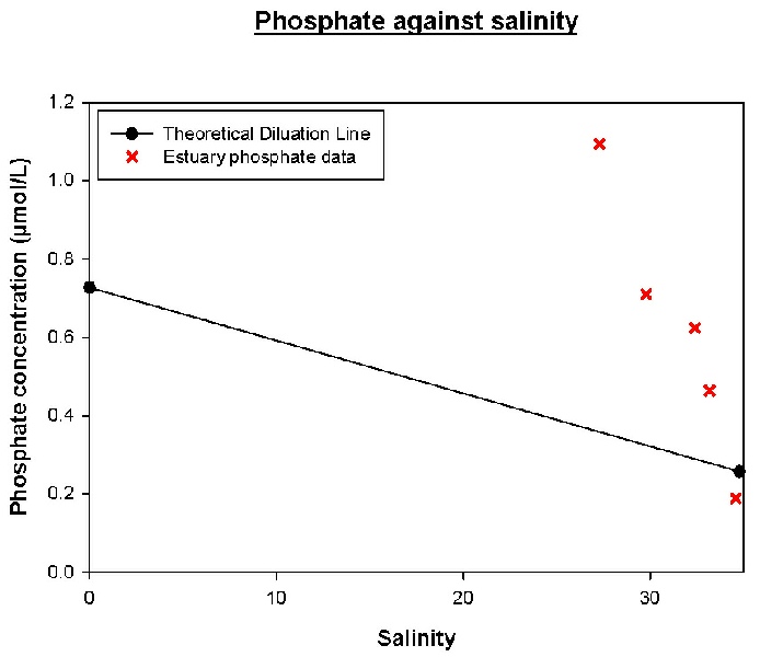
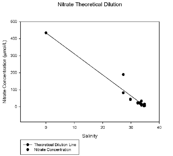
Figure 10
Dissolved Oxygen Measurements
Methods
The Winkler method was used to analyse the dissolved oxygen concentration in the water column at specific stations (1,2,3,4,6,7) along the estuary. Samples were collected from three depths at stations 1 and 2 and two depths at stations 3,4,7 and at one depth from at station 6 by Niskin bottles. Samples were stored in the glass stoppered bottles to minimise the exposure to the open atmosphere, preventing contamination. Two reagents alkaline iodine and manganese chloride were added and samples were later incubated for approximately 24 hours. After that period, 1 ml of sulphuric acid was added and the samples were continuously mixed. The solution was titrated with sodium thiosulphate, using an auto-burette to achieve precise readings. The dissolved oxygen concentration was calculated based on the assumption that 1mol oxygen is equivalent to 4 mol of sodium thiosulphate.
Interpretation
Station 1 shows supersaturated oxygen levels (106.5%) at water surface. This might correlate to the high number of phytoplankton we collected at that station (fig 17). High primary productions usually portray high oxygen levels during the day due to photosynthesis. At station 2, oxygen saturation decreases with increasing depth (fig 16). Reasons for this could include high zooplankton levels (consuming oxygen through respiration), and decomposition of material by bacteria in mid to lower layers in the water column. Station 3 and station 4 show quite similar patterns of plots with small increases (1.4% and 3.1%), which appear to be the most stable in terms of oxygen saturation levels. It is possible that the amount of consumed oxygen is almost balanced by processes that give off oxygen at all the depths. Despite the high temperature at station 7, oxygen levels at station 7 are low compared to the other stations. This probably due to high number of zooplankton (fig 18) that reduces oxygen concentrations by decomposition and respiration.
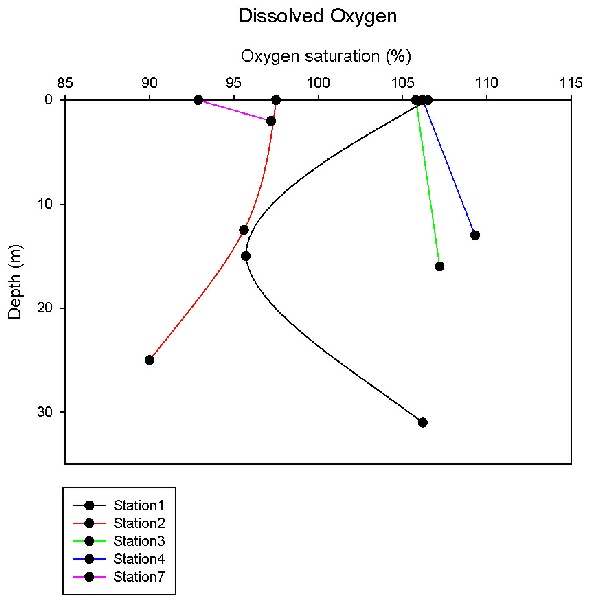
Figure 16