Disclaimer: These findings are the personal interpretation of the students involved and do not reflect the views of the University of Southampton, the National Oceanography Centre or Falmouth Marine School.


Calculations
Residence Time
Tres=(f Vtotal)/R = (1-(Smean/Ssea))Vtotal/R
Vtotal= 126341773m3
R= River Fal at Tregony- 0.8m3s-1
River Kenwyn at Truro- 0.1m3s-1
River Kennal at Ponsanooth- 0.18m3s-1
Carnon River at Bissoe- 0.38m3s-1
Rtotal= 1.46m3s-1
smean= mean salinity from Station1 to Station 7=33.3864
ssea=35.21747
Tres= (1-33.3864/35.21747)x126341773m3
1.46m3s-1
= 4499258.08s
= 52days 2hours
Flushing Time
T = Vestuary/Vprism ×Ttidal
Ttidal= 12.3667hours
Aestuary= 24820000m²
Vestuary = Total Estuarine Volume = Aestuary mean depth
Vprism=Aestuaryh
h=Tidal range(HW-LW)
mean depth= (Hs1+Hs2+Hs3+Hs4+Hs5+Hs6+Hs7)/7=(35m+27.5m+19.2m+18.4m+11.6m+9.5m+5.5m)/7=1 8.1m
h=5.2m-0.2m=5m
T =(18.1/5)12.3667=1day 21hours
Rossby Number
Rossby No.= U/(L x f)
Coriolis Parameter 'f '=2Ω sinφ
f = 2 x 7.3 x 10-5 x Sin(50o )=.46 x 10-4 x 0.766 = 1.12 x 10⁻⁴
Area 1 (lower estuary): U = 0.08ms-1 L = 4000m Rossby Number = 0.179
Area 2 (upper estuary): U = 0.15ms-1 L = 3000m Rossby Number = 0.448
Rossby Radius of Deformation
Rd= (gxZ)1/2 /f
g = 9.8ms-2
Average depth ‘Z’ = 25m
Rd = 140km
ADCP
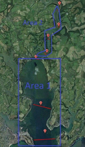
Figure 1:
Start Time = 08:29:35 Duration = 847.30s Flow speed = 0.211
Flow Direction = 164.15 Total Q = 3896.93 m3s-1
Figure 2a and Figure 2b:
Start Time = 09:37:52 Duration = 650.67 s Flow Speed = 0.159 ms-1
Flow direction = 212.27 Total Q = 3136.56 m3s-1
Figure 3:
Start Time = 10:26:09 Duration = 175.62 s Flow Speed = 0.370 ms-1
Flow Direction = 212.18 Total Q = 873.10 m3s-1
Figure 4:
Start Time = 10:49:19 Duration = 119.11 s Flow speed = 0.202 ms-1
Flow Direction = 248.54 Total Q = 556.70 m3s-1
Figure 5:
Start Time = 11:24:27 Duration = 136.46 s Flow speed = 0.168 ms-1
Flow direction = 194.98 Total Q = 281.02 m3s-1
Interpretations
Results
The transects from stations 1 and 2a show the velocity of the outgoing ebb flow being slightly greater on the western sides than the eastern sides (figures 1 and 2a). By Station 3 this trend decreases and throughout stations 4, 5, 6 and 7 flow varies more with the local topography.
The Stick Ship Track for Station 1(Figure 2b) shows the potential effects of the Coriolis Force on the outward ebb flow, with the flow in the middle of Area 1 flowing in a South Westerly direction, as opposed to directly south out the estuary.
Coriolis Effect
Any movement in the Northern hemisphere is acted upon by the Coriolis force 90o to the right of the direction of motion. This concept could be applied to the observations from stations 1, 2 and 3 to explain the increased velocities on the western sides.
Two factors that determine the magnitude of the Coriolis Effect on a body of water are the length scale and velocity of the water mass. Taking these parameters into consideration we can calculate the Rossby number. A high Rossby number suggests the Acceleration Terms in the equation are significantly larger than the Coriolis Effect and therefore the Coriolis Effect can be neglected. A low Rossby number however suggests these Accelerations Terms are small and therefore the Coriolis Effect is relevant. (Knaus 1997)
Calculating the Rossby number for the region where the velocity is faster on the Western side (Area 1) and the region where this is not observed (Area 2) gives values of 0.179 and 0.448 respectively. Considering the lack of wind and the fact the Rossby Number for Area 1 (0.174) is small, the Coriolis Effect could be the reason behind the slight 0.1 ms-1 increase in velocity from the Eastern to the Western side. The value for Area 2 (0.448) is 2.5 times larger than in Area 1, thus the Acceleration Factors are 2.5 times greater here than in Area 1, and the Coriolis Effect could be considered negligible.
The Rossby Radius of Deformation defines the length scale where one can expect to observe the effect of a kelvin wave (Knaus 1997). The Rd value for Area 1 suggests the water would have to flow a distance of 140km for geostrophic balance to be notable. As the length scale of Area 1 is only 4km, one would not expect to be able to witness the geostrophic balance here, and one could argue Coriolis is not significant.
However as stated by Knaus 1977, the earth’s rotation cannot be completely ignored in estuaries. As in broad estuaries with weak tidal currents there is a tendency for the outflow to hug the right side of the estuary in the Northern Hemisphere and the incoming tidal flow to hug the left side. This often results in slightly higher salinities on the right hand sides, and slightly lower salinities on the left. As the variation in velocity is small (0.1ms-1) it would be fair to consider the Coriolis Effect is present.
If we could sample the estuary again, ideally we would use the CTD to sample both sides of Area 1 as opposed to just the middle, to look into the possibility of differences in salinity and density across the estuary.
Analysis of Residence and Flushing Time
The values shown are taken from the CTD data. The rate of estuarine discharge was taken from the Centre for Ecology and Hydrology site at Wallingford (See useful links in References).
The residence time calculated above provides an idea of the flushing time of the Fal Estuary due to river discharge rates. The Residence Time calculated using the prism method gives an idea of the flushing time of the Fal Estuary due to tidal flow as opposed to riverine discharge.
The residence time of the estuary is relatively long, due to the sea having a far greater influence than the river input. From the ADCP data taken the same day on a flooding tide, the incoming volume was 1180.874 m3s-1 (+/-10%) at 08:33GMT at 0.185 ms-1 while the average riverine flow into the estuary for June is 1.46 m3s-1, representing a much smaller value. The high residence time means that any pollutants will stay in the estuary for an average of 52days 2hours before entering the ocean.
The lower flushing time suggests that the tidal cycle has a much larger effect on estuarine flushing than tidal discharge. This hypothesis is supported by the high average salinities found at the most riverine stations.
It is not highly accurate due to the way different parameters are measured. It was often found that a small change in any part of the data produced a large change in the result.
Richardson Number
The Richardson Number is used to quantify the extent of density stratification and mixing for each CTD profile collected for each station (fig 6). A Richardson Number below 0.25 indicates the presence of shear instabilities whilst a value greater than 1 indicates laminar flow (no mixing).Temperature of most stations shows a gradual change with depth with no defined thermocline. Salinity also demonstrates little change with depth. Both of these patterns are characteristic of a well-mixed water column, which can be confirmed using Richardson Numbers of all the seven stations.
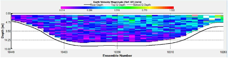
Figure 4
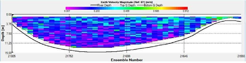
Figure 5
Temperature
Results
The surface temperature increases by approximately 3.25°C along the length of the estuary, from Station 1 to Station 7 (fig 7). At Station 1 there is a decline in temperature of 0.5°C from the surface to depth. A decline can also be seen at Stations 2 to 6, but this is only very slight. Station 7 shows no change in temperature.
The disparity between profiles for a single station could be due to the drifting of the boat causing the CTD to move from it’s original position.
Discussion
The change in temperature from the surface to depth is due to the colder, denser seawater coming into the estuary and flowing underneath the warmer river water. Despite the mixing between the two layers, the colder water will still sink to the bottom. The surface water is also warmed by solar radiation.
Salinity
Results
Moving up the estuary, the salinity decreases by approximately 7.5 salinity units across the seven stations (fig 8). At the earlier stations, the depth profiles are visibly uniform, with Stations 1 and 2 being almost identical. At Station 5 a slight halocline has developed, which is present from that point onwards. From Station 6 to Station 7 there is a salinity decline of 4 salinity units, which is the largest difference between two stations.
Again, the disparity between profiles for a single station could be due to the drifting of the boat causing the CTD to move from it’s original position.
Discussion
At the mouth of the estuary the depth profile shows a constant salinity for the whole of the water column, which shows that at this point the estuary is well-mixed. There are small increases in salinity from the surface to depth at Stations 5 to 7, which show the beginning of a salt wedge, where the denser, more saline seawater flows up the estuary underneath the lighter, fresher river outflow.
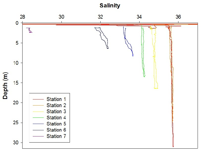
Figure 8
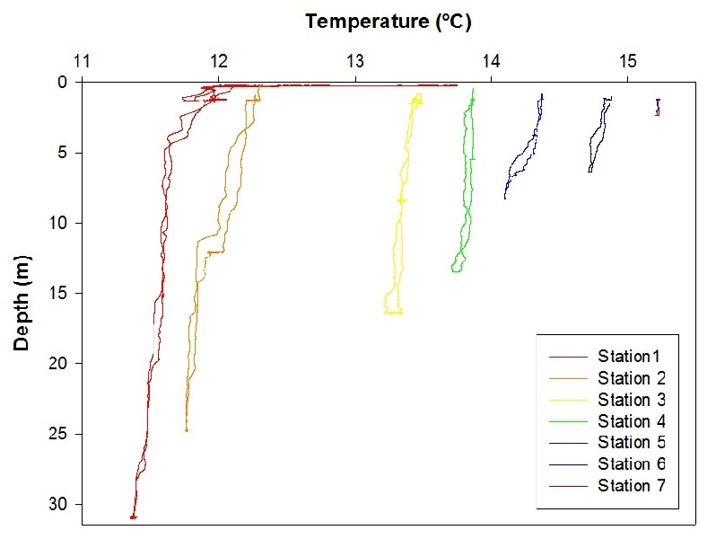
Figure 7
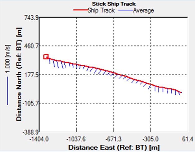
Figure 2b
Figure 1
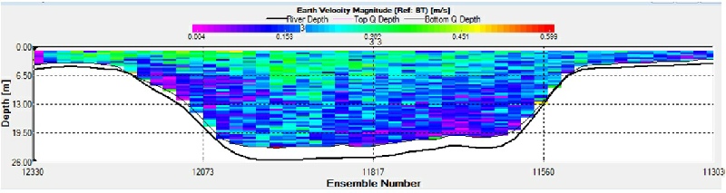
Figure 2a
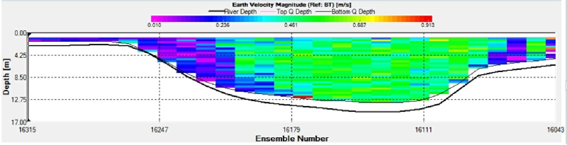
Figure 3
Physical Factors
Turbidity
Interpretation
By looking at figure 9, it can be seen that turbidity decreased slightly, by a value of approximately 2NTU overall, moving up the estuary. This could be due to the wave action near to the mouth of the estuary affecting the turbidity within this area. Throughout the water column turbidity remains constant with very little variation except for stations 5 and 6, where negligible variations can be seen. This could be due to natural factors such as tides, seabed friction and possibly large organisms being active near the CTD when recordings were taken. Again, these can only be assumptions, and further investigations would need to be under taken to prove these hypotheses.
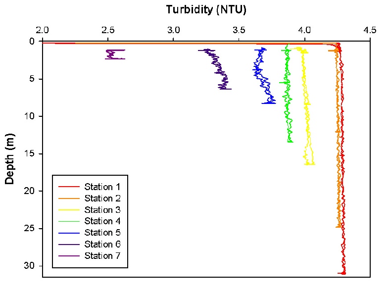
Figure 9
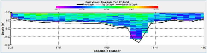
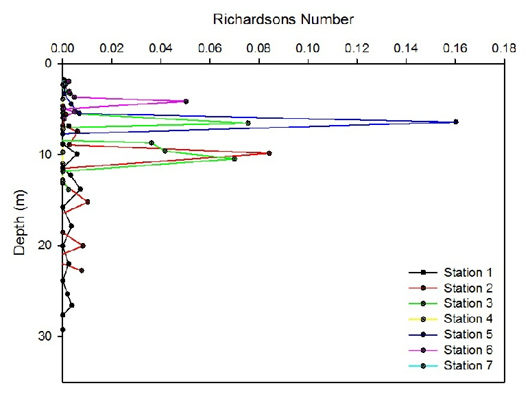
Figure 6