Falmouth 2015 -
Irradiance is seen to decrease exponentially with depth at all stations, from approximately 1200PAR at the surface down to 0PAR at ~30m. Station 3 has the lowest attenuation coefficient (K) (See table 3) which is illustrated in figure 3 as the irradiance curve can be seen decreasing at a lower rate than the other stations. Station 1 and 2 have similar attenuation coefficients, but station 1 has a significantly sharper decrease in irradiance at shallow depths (between ~1.1m and ~1.6m) from approximately 750PAR to 300PAR. Station 2 does not exhibit such a sudden decrease, and although a lot of fluctuation is seen, overall light attenuation is similar due to the fact that light attenuation at station 1 slows after the initial sharp drop. Due to light being attenuated quickest in surface waters at station 1, lower phytoplankton abundance is expected here in comparison to the other stations.
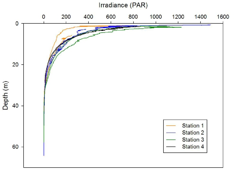
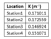
Figure 2: Irradiance vs Depth at all stations (Click to enlarge).
Table 2: Attenuation Coefficient (K) at each station.
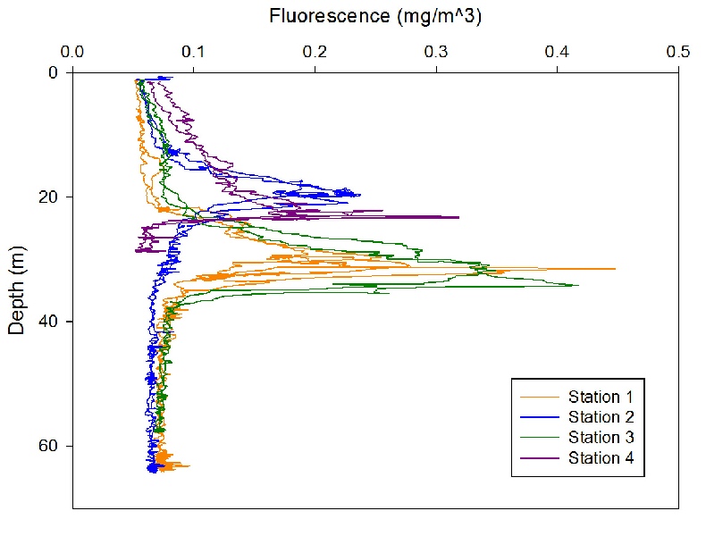
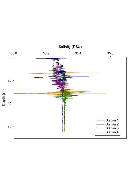
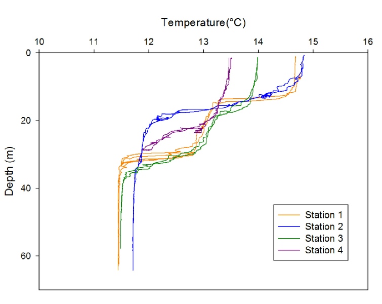
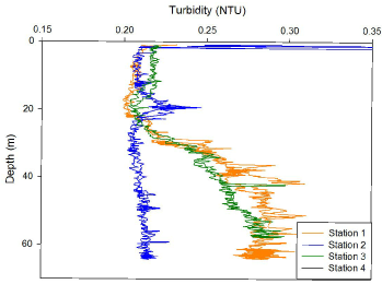
Figure 5: Fluorescence vs Depth at all stations (Click to enlarge).
Figure 3: Salinity vs Depth at all stations (Click to enlarge).
Figure 4: Temperature vs Depth at all stations (Click to enlarge).
Figure 6: Turbidity vs Depth at all stations (Click to enlarge).
Physical
Data collected from the CTD & ADCP deployed from RV Callista.
Salinity was shown to be fairly consistent between the four stations. The profiles are hard to study due to a large number of salinity spikes however you can observe that generally at all stations the surface 20m of the water column was fresher by ~0.05psu than the deeper waters. This small freshening is likely due to freshwater river input from the Fal estuary. Station 1 and station 3 appear to have marginally higher salinities than station 2 and station 4, however the difference is so small that we have considered it as being insignificant. (See Figure 3)
Tidal fronts develop between stratified regions and tidally mixed regions, and stratification is determined by density. As at all stations salinity was fairly constant with depth, we can assume that density in this region is dominated by temperature (controlled mainly by solar heating). Surface water temperatures will be higher in the stratified offshore waters than in the tidally mixed waters.
Station 1 shows strong 2 step stratification with a thermocline of 1.7⁰C at 18m and
a second thermocline of 1.3⁰C at 34m. (See figure 4) As we moved further offshore
station 2 showed strong stratification with a single thermocline of 3.0⁰C between
10m and 20m. At station 3, positioned near station 1 but slightly inshore (see Figure
1-
Comparing the surface temperatures between each station you would expect those in mixed waters to be cooler and those in the stratified waters to be warmer as waters held at the surface by the stratification are further warmed by solar heating. From our survey we found station 1 and station 2 to have the highest surface water temperatures of ~14.7⁰C , station 3 to have a surface temperature of 14⁰C and station 4 to have a temperature of 13.5⁰C. These observations support the idea that station 1 and 2 were in stratified waters, station 3 was near the front and station 4 was in the mixed waters.
Fluorescence is an indication of the presence of phytoplankton. Station 1 and station 3 showed a large peak of ~0.4mg/m^3 at ~35m. (See figure 5) The peak at Station 2 was smaller at 0.24mg/m^3 at a depth of 20m. The peak at station 4 was also less than station 1 and 4 at 0.3mg/m^3 at a depth 25m. This indicates that higher levels of phytoplankton are found near station 1 and station 3, which is the area in which we predicted where the tidal front was. The peaks of fluorescence are found at a similar depth to that of the thermocline at most stations, suggesting deep chlorophyll maxima. This forms where phytoplankton bloom in a deeper region where there is enough light for photosynthesis, but there is also a continuous supply of nutrients from deep waters (as surface nutrients have been depleted by previous blooms) (See also Figure 9 to support this theory).
Turbidity was similar at all stations with values of ~0.22NTU down to depths of ~25m. Below this depth, turbidity remains constant at station 2 down to 60m and the maximum depth of station 4 is reached. However, turbidity at station 1 and 3 increased below 25m to values of ~0.28NTU.
We see that for station 2, turbidity and fluorescence (Figure 5) peak at the depth
of the thermocline. This correlates with an increase in chla and oxygen concentrations
(Figures 9 & 10 on Offshore-
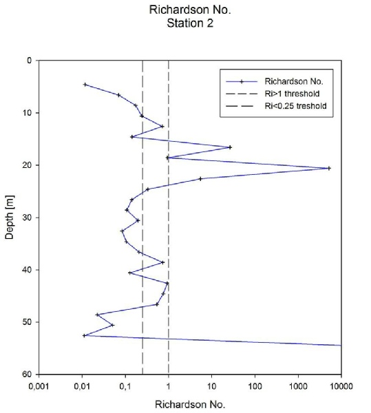
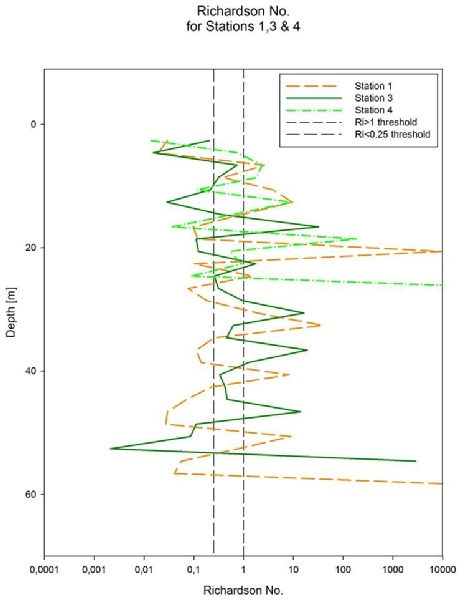
Richardson number is a measure of the ratio of buoyancy forcing to mixing in the form of flow gradient. Therefore it is a useful measure of the water column stability and gives information about the likelihood of internal waves resulting in turbulence. If Ri is small, this means that shear velocity is strong enough to overcome stratification, meaning that turbulence and mixing is likely to occur. For large Ri, cross thermocline stratification is generally suppressed.
For station 2, which is in the stratified region, Ri only reaches high levels around the thermocline, which is expected as this is where stratification was strongest. At all other depths, Ri is either smaller than 0.25 or in the intermediate region, suggesting that convective mixing may be happening on either sides of the thermocline. Velocity values are clustered around 0.4m/s for the whole water column.
Station 1, 3 and 4 all exhibit a similar chaotic pattern for Ri. Clear spikes appear at the depth of the thermocline but the rest of the vertical profile shows variation following velocity magnitude changes whilst direction variations are accounted for. However, overall velocity magnitudes for stations 1, 3 and 4 are smaller than at station 1 but exhibit larger horizontal variability. The reason for this could be a higher influence of bottom friction, seeing as stations 1, 3 and 4 display very low velocities close to the seafloor.
Generally speaking, this fluctuating pattern in Ri profile indicates a less stable water column, which agrees with the previous statement concerning high mixing locations.
Figure 7: Richardson Number against depth at Station 2 (Click to enlarge).
Figure 8: Richardson Number against depth at Station 1, 3 & 4 (Click to enlarge).
Transects of backscatter were recorded from the bottom mounted ADCP on board Callista
and then extracted using WinRiver software. Data was collected at each Station 1-
Hence the transects of backscatter were used to infer sub-
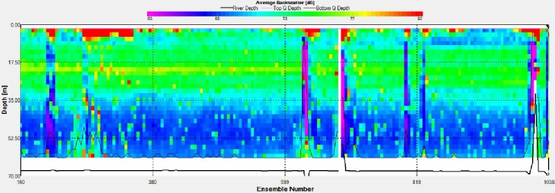
Station 1: From the CTD temperature profile there was a strong double thermocline at 13m and at 30m, this can be seen, particularly towards the right of this picture, as backscatter occurs in two bands at the equivalent depths, though there is a strong signal throughout the depth of the thermocline. (Figure 9)
Furthermore, looking at the fluorescence profile from the CTD data shows a peak at ~30m indicating high phytoplankton concentrations at this depth. But given that most backscatter occurs above this depth it may be indicative of zooplankton grazing from above or else the prevalence of zooplankton species which prefer shallower water although this will require further research.
Figure 9: Backscatter signal at Station 1 (Click to enlarge)
Figure 10: Backscatter signal showing the transect between Stations 1 & 2 (Click to enlarge)
Between Stations 1 & 2: The pattern of backscatter between stations 1 & 2 heading
offshore shows a shallowing of the thermocline being focused between 10-
Although there is a large level of noise inherent in shipborne ADCP backscatter when the boat is moving (Heyward et al. 1991) and this is evident in all the transects between stations here, it is still possible to get a good picture of the first ~20m of water although care is of course necessary
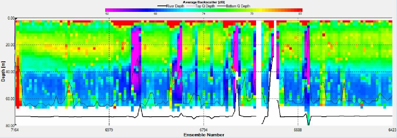
Figure 11: Backscatter signal at Station 2 (Click to enlarge)
Transect to Station 3: Heading back in shore we were looking for the edge of the front and the apparent weakening of the backscatter signal led us to try an investigative CTD profile. But clearly from the backscatter when stopped at the station itself there was still a strong signal from the double thermocline with two nearly discrete bands of backscatter at approximately 19 and 35 meters again correlating well with the CTD temperature profile. Hence from the profiles and the pattern of backscatter it was decided not do any sampling and to head further toward shore.
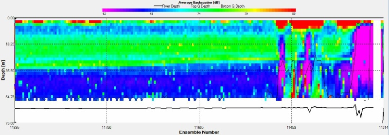
Figure 12: Backscatter signal showing the transect between Stations 2 & 3 (Click to enlarge)
Figure 13: Backscatter signal at Station 3 (Click to enlarge)
Transect to Station 4: The ADCP transect heading towards station 4 showed the characteristic rise of the thermocline, and hence zooplankton and backscatter, to the surface that we had hoped to see and is expected at a front. Within the well mixed waters beyond the front there is little structure to the pattern of backscatter and hence zooplankton with low readings at all depths except in the surface waters which is only a result of the gently motoring vessel maintaining position at station.
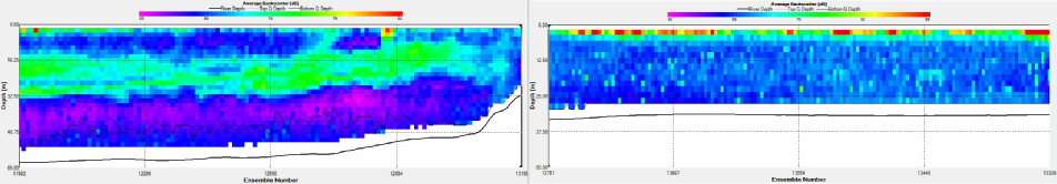
Figure 14: Backscatter signal showing the transect between Stations 3 & 4 (Click to enlarge)
Figure 15: Backscatter signal at Station 34 (Click to enlarge)
Flagg, C.N., & Smith, S. L. (1989). On the use of the acoustic Dopler current profiler
to measure zooplankton abundance. Deep Sea Research Part A. Oceanographic Research
Paper, 36(3), 454-
Heywood, K. J., Scrope-
Disclaimer: The views expressed here are not associated with those of the National Oceanography Centre Southampton or the University of Southampton.