Offshore: Physical

This page looks at:

• Temperature Data
• Density Data
• Salinity Data
• Attenuation Coefficient
• Flow Velocity
• Richardson Number

Temperature Data

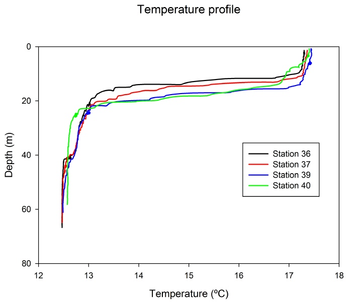
Figure 1: Temperature vs Depth for all stations

Figure 1 shows the temperature depth profile from all stations offshore. According to the figure you can see a thermocline at all stations, which is expected since in the summer the longer exposure to the sunlight and the warmer temperature increases the surface temperature, creating a stratified water column. While in the winter the water column is expected to be well-mixed and colder. The variations between the stations is due to the time interval of one hour between each measurement, allowing the later stations to have a longer exposure to the sun, consequently warming up the surface and increasing the depth of the thermocline.

Density Data

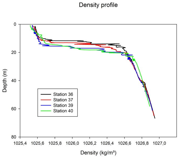
Figure 2: Density vs Depth for all stations

This density depth profile shows a pycnocline at the same depth as the thermocline seen in figure 2, however there is an inverse relationship with the temperature. This was expected since the water is stratified due to the warmer temperatures in summer.

Salinity Data

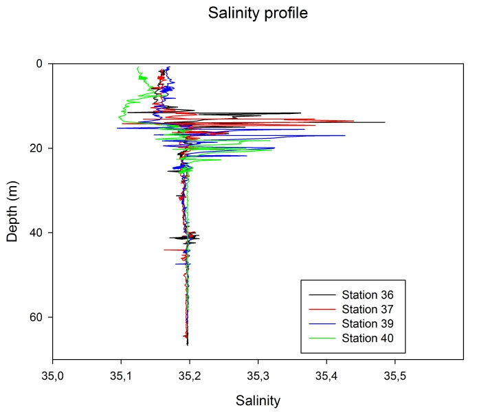
Figure 3: Salinity vs Depth for all stations

The salinity profile (figure 3) shows spikes as a result of the time lag of temperature measurement and conductivity.  It is not possible to make a full analysis of the salinity with this graph alone, however after the depth of about 30 meters the graph tends to stabilize and it is noticeable that overall all the stations shows similar salinity.

Attenuation Coefficient

The attenuation coefficient was calculated using the formula k*D=1.46 (Holmes, 1970) (table 1), where k is light attenuation coefficient and D is the secchi disk depth. Euphotic zone was calculated as three times the secchi disk depth.

The water visibility can be affected by both water turbidity and weather (cloud coverage). In the ocean, it is expected to have clear water with less turbidity than those in the estuary. Due to that, the values of Secchi disk depth are more influenced by the weather than the water turbidity. It is possible to observe in table 1 that higher secchi disk depth was obtained in stations with less cloud coverage and consequently deeper euphotic zones as well.

Flow Velocity

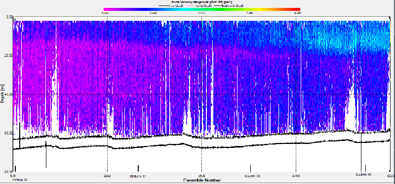
Overall the water velocity shows a similar pattern in all transects (figure 5), with a faster water mass in the surface above the slower water mass observed below. However, in the last two transects the velocity of both masses increases, but still presenting the same pattern of a faster mass in the surface.

Figure 4: Velocity obtained by ADCP between stations 36 and 40.

Richardson Number

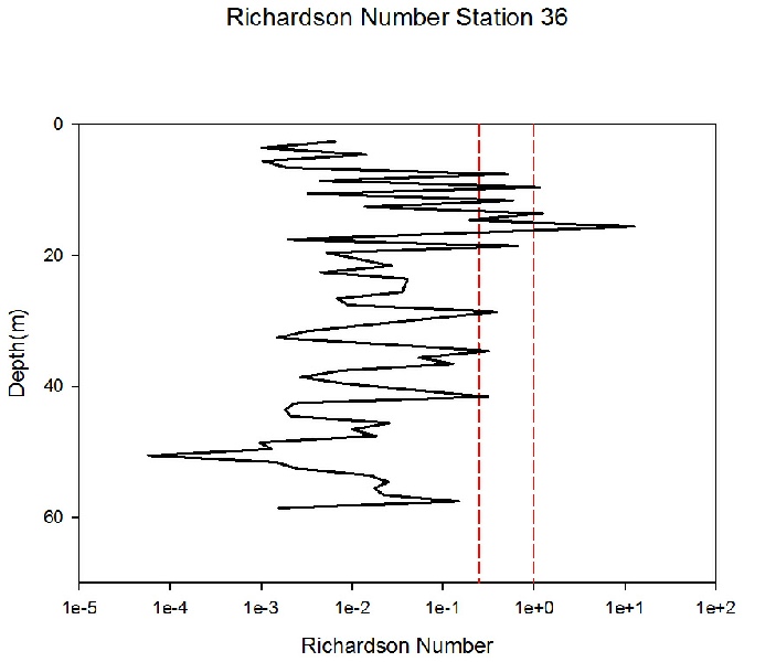
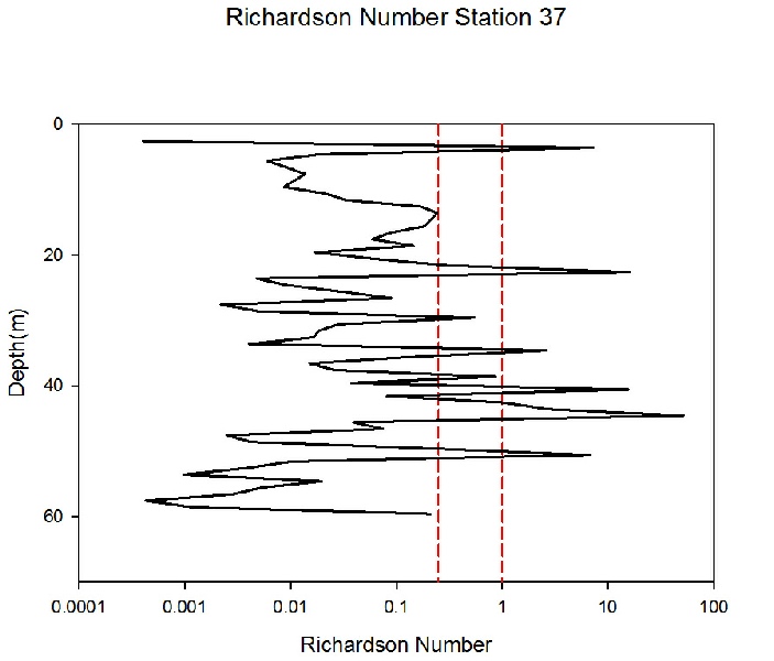
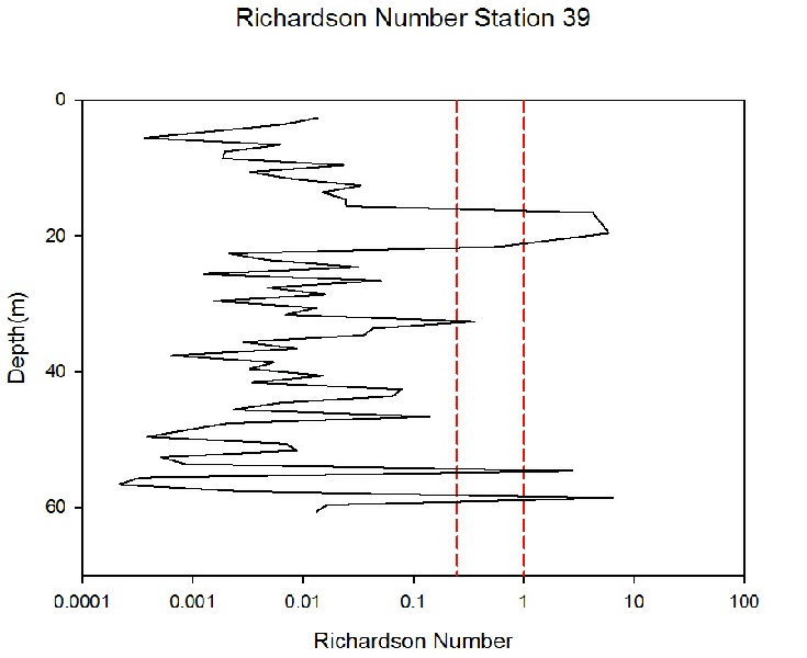
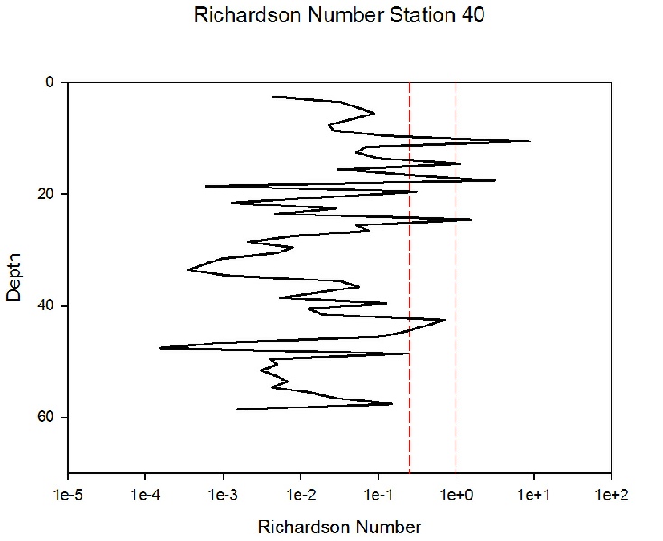
Assuming values found above 1 are laminar (Abarbanel et al, 1984) and below 0.25 are turbulent (Miles, 1961), these are represented as red lines in figures 5, 6, 7 and 8. It is possible to observe in the figures that there is a predominance of turbulent flow. In all stations it is noticeable some peaks of laminar flow around depth 15 to 20 meters.

References:

Abarbanel, H. D., D. D. Holm, J. E. Marsden, and T. Ratiu, (1984). Richardson number criterion for the nonlinear stability of three-dimensional stratified flow. Phys. Rev. Lett., 52, 2352–2355.

Holmes, R. W. (1970). The Secchi disc in turbid coastal waters. Limnology and Oceanography, 15, 688-694.

Miles, J. W., (1961). On the stability of heterogeneous shear flows. J. Fluid Mech., 10, 496–508.

Falmouth, 2014