Figure 9.
Figure 10.
Figure 11.
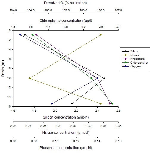
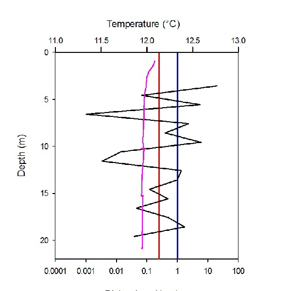
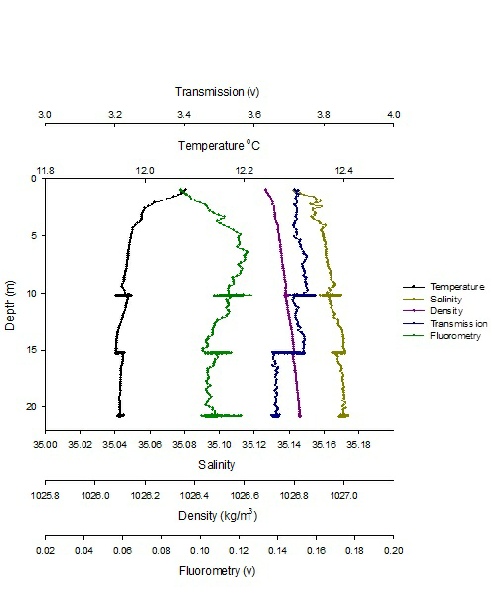
Figure 2.
Figure 3.
Figure 4.
Click on the figures to see an enlarged version with figure label.
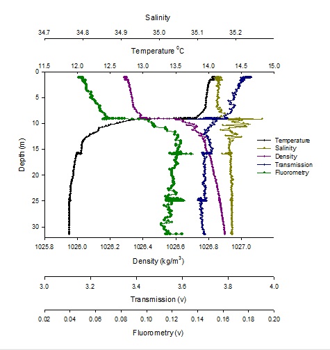
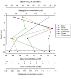
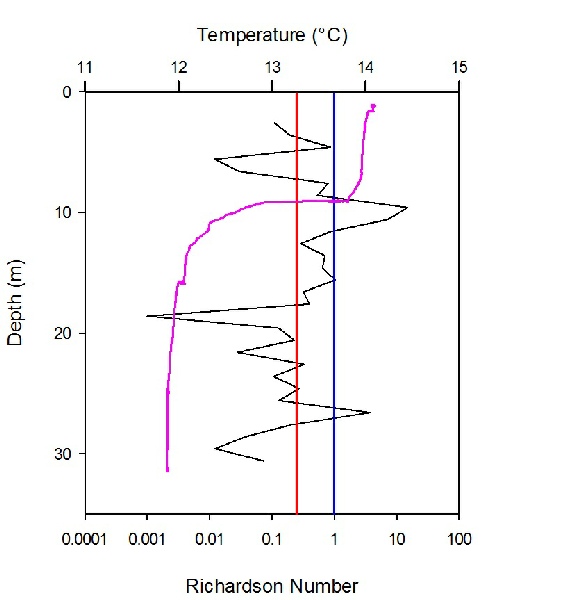
Figure 5.
Figure 6.
Figure 7.
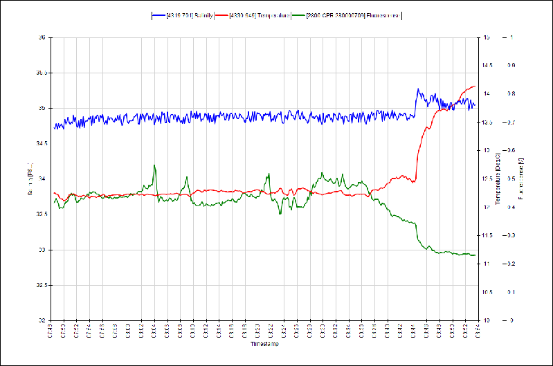
Figure 8.


|
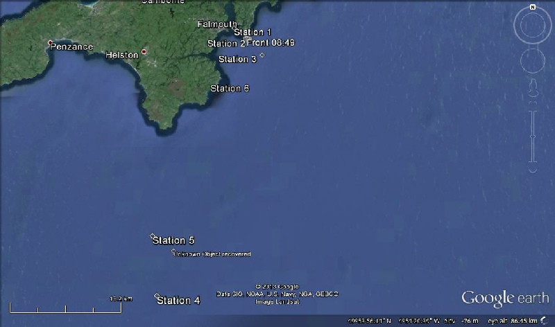
Key for Offshore Map: Front 08.49: Location at 08:49 UTC, (where the vessel crossed a detectable front; Lat: 50° 07.698, Long: 004° 59.448) Unknown Object recovered: Lat: 49° 45.146 Long 005° 09.739 Station 1: Lat: 50° 08.902 Long: 005° 01.613 Station 2: Lat: 50° 07.540 Long: 004° 58.800 Station 3: Lat: 50° 05.700 Long: 004° 56.831 Station 4: Lat: 49° 40.974 Long: 005° 11.793 Station 5: Lat: 49° 46.552 Long: 005° 13.004 Station 6: Lat: 50° 01.679 Long: 005° 01.589 |
Vessel: R.V. Callista
Introduction:
Samples were collected at various locations(see Figure 1) starting at Black Rock and ending to the South of The Lizard. En route to stations the ADCP and salinothermograph collected transect data related to currents, temperature, salinity and fluorescence. This data was used to indicate where the CTD should be deployed.
Methods:
CTD
The CTD was deployed from the back of the R.V. Callista. On the downward profile, data was collected for temperature, salinity, irradiance and fluorescence. This profile was used to indicate where to fire the Niskin bottles to collect samples within the differing water masses on the upward profile, whilst still collecting data on the various parameters.
Zooplankton Net
A 60cm diameter, 200µm mesh zooplankton net was deployed from the back of the ship
using an on-
Secchi Disk
At all 6 stations the secchi disk was deployed. At some of the stations the deployment was repeated 3 times so that an average could be calculated. The secchi disk depth is then multiplied by 3 to calculate the depth of the euphotic zone.
Labs:
All instruments used when handling water samples were washed with an aliquot of the sample before use to ensure no contamination occurred.
Oxygen sampling: During collection of oxygen samples care had to be taken to prevent the introduction of oxygen from the external environment. Water samples were collected in glass bottles and Winkler reagents, manganous chloride and alkaline iodide, were added to the water samples before storage in cold water as outlined in Grasshoff et al7.
Phytoplankton sampling: 100ml of water were measured and transferred into labelled
glass bottles, which contained Lugol’s iodine in order to stain and preserve the
phytoplankton within the sample. In the lab the sample was then reduced to 10 ml
using vacuum filtration. The samples were then placed in a sample vial and analysed
using a microscope. 1 ml of the sample was placed on a Sedgewick-
Nitrate and Phosphate: Onboard 50ml were measured and filtered using a microfiber filter in to labelled glass bottles and stored in a cooler. In the lab dissolved nitrate was measured using the procedure outlined in Johnson and Petty8. The phosphate concentration was measured using the procedure outlined by Parsons et al9.
Dissolved Silicon: 50ml of the water sample were filtered through a microfiber filter into plastic bottles and were stored in the cooler box. Analysis of the dissolved silicon is outlined by Parsons et al9
Chlorophyll: Chlorophyll which collected on the filter were retained and stored in test tubes, containing acetone, in the fridge. The concentration was then measured in the lab using the flurometer as outlined in Parsons et al9.
Zooplankton: A sample of the water from the Niskin bottle was directly transferred into a 1L plastic bottle and 10% Formalin solution was added in order to preserve the sample. The zooplankton contained in 10ml were then counted under the microscope using a Bogarov tray. These counts were used to calculate the number of zooplankton that would be present in a cubic meter of seawater.
Figure 1. A map to show the stations sampled during the offshore research cruise. The point at which the front was crossed is also labelled.
Discussion:
Station. 1
Station 1 showed no definitive thermocline, pycnocline or halocline due to the water
column being well mixed which was also reflected in the ADCP data. At the surface
the fluorometer recorded chlorophyll minima due to photoinihibtion, however below
3 metres the fluorescence level remained constant throughout the water column (figure
2). The low chlorophyll levels but high nitrate levels at the surface (figure 3)
reinforce the concept of photoinhibition close to the surface. The high nitrate levels
are due to the station being situated at the mouth of the estuary, therefore it is
heavily influenced by estuarine processes such as hyper-
Station. 2
Station 2 is located just outside a tidal front as detected by the thermosalinograph (figure 5). The downcast at station 2 showed strong evidence of a thermocline, pycnocline and halocline, indicative that the water column was highly stratified (figure 6). The silicon concentration increased with depth, remaining high beneath the thermocline. There appeared to be a delayed phytoplankton response to the nutrient concentrations as the chlorophyll levels remained low at 10m, despite the peak in nitrate and phosphate concentrations. It is therefore likely that the high nutrient levels were introduced to the Station 2 on the outgoing tide. The chlorophyll maximum was recorded at 24.6m, (figure 7) however phytoplankton samples did not reflect this (figure 22). This is due to the samples not being fully representative of 24.6m because of the sampling method. A high attenuation coefficient would suggest that the 1% light level would reach below this point, however Secchi disk data determined the level to be at 23.8m.
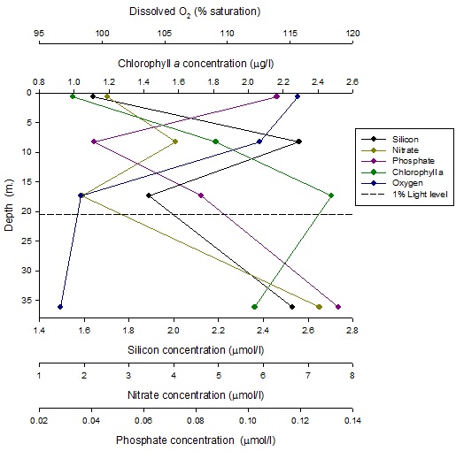
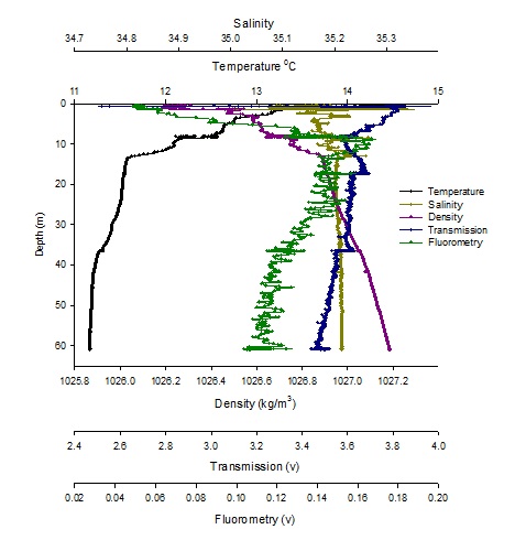
Station. 3
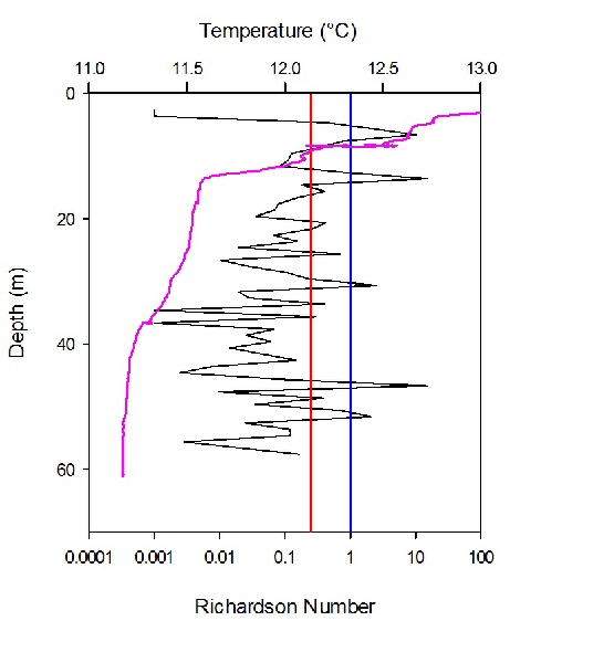
Station 3 was partially mixed, with a less defined thermocline and pycnocline in comparison to station 2 (figure 9). There is a large peak in fluorometric data at 10m suggesting high chlorophyll concentrations. This is not mirrored in the chlorophyll data (figure 10) however the chlorophyll data from the laboratory analysis was deemed to be more accurate. The chlorophyll maximum occurred at the same depth as the oxygen minimum at around 17m. High turbidity levels were recorded in the surface waters (figure 9) however this corresponds to a chlorophyll minimum (figure 10), suggesting that the turbidity is caused by abiotic factors such as turbulence. The highly unstable water column (figure 11) shows a highly variable Richardson Number with depth, with most readings showing a Richardson Number below 0.25, suggesting instability. Station 3 is a highly dynamic station, located on or close to a tidal front. The surface waters showed nutrient limitation as both the nutrient and the chlorophyll concentrations are low (figure 10). With depth the nutrient levels increased as a result of oceanic inputs. The silicon and nitrate concentrations showed a positive correlation suggesting that they are both consumed by the phytoplankton. Upon further examination of the phytoplankton data (figure 22) there are an abundance of diatom species, which accounted for the silicon profile.
Click here to see the continuation of the offshore discussion.