Disclaimer: The views and opinions expressed are solely representative of the contributors, and are not necessarily condoned or supported by the University of Southampton and/or the National Oceanography Centre Southampton.

OFFSHORE - PHYSICAL

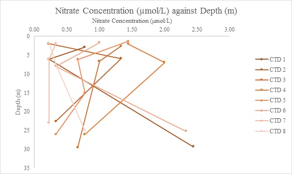
Figure 1: Nitrate concentration (µmol/L) with depth (m) time series. CTD 1 was taken at 09:55 and CTD 8 was taken at 15:55 UTC.

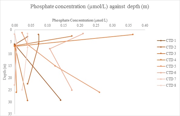
Figure 2: Phosphate concentration (µmol/L) with depth (m) time series. CTD 1 was taken at 09:55 and CTD 8 was taken at 15:55 UTC.

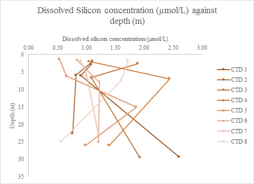
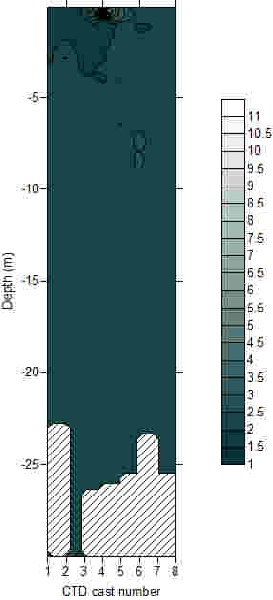
Figure 3: Dissolved silicate concentration (µmol/L) with depth (m) time series. CTD 1 was taken at 09:55 and CTD 8 was taken at 15:55 UTC.

There were large changes in nitrate concentration with tide. The main factors responsible for these changes are tides and riverine input. A decrease in nitrate with depth may be due to uptake by phytoplankton, therefore less nitrate reaches further down the water column. Force 5 Easterlies during the sampling period may have contributed to lower concentrations at surface than at depth; as wind action increases vertical mixing, nitrate may be mixed to greater depths.

The data shows that at most times throughout the day phosphate decreases rapidly from surface to 7m (the Shallow Chlorophyll Maximum). This is due to uptake by phytoplankton. As the phytoplankton die and aggregates fall further down the water column, phosphate dissolves back into the water. This is why there is an increase from 7m towards the bottom of the water column. There is a general trend of an increase in phosphate towards low tide (CTD 6), the concentrations then decrease during the flood tide.

The silicon profiles are very irregular, this may have been contributed to by the weather conditions on the day of sampling. It is possible that wind driven mixing from Force 4-5 easterlies caused this in addition to the the drift of the vessel during CTD deployment.

Temperature (oC)

Salinity

Chlorophyll (µmol/L)

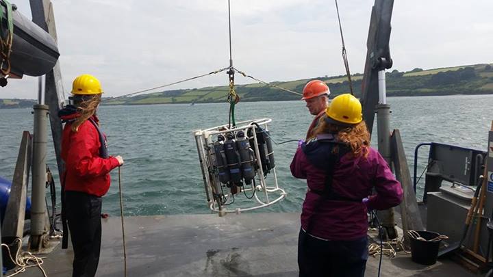
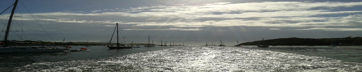
Figure 4: Undergraduates deploy the CTD at the Carrick Roads sampling station.

Figure 5 (left): Time series of temperature fluctuations throughout water column from 09:54 UTC (CTD cast 1) to 16:33 UTC (CTD cast 8).

Figure 6 (centre): Time series of salinity fluctuations throughout water column from 09:54 UTC (CTD cast 1) to 16:33 UTC (CTD cast 8).  

Figure 7 (right): Time series of chlorophyll fluctuations throughout water column from 09:54 UTC (CTD cast 1) to 16:33 UTC (CTD cast 8). Note: The concentrated black spot between cast 3 and 4 is showing high chlorophyll. It appears black due to a high concentration of contour lines as the chlorophyll is changing so rapidly.

The temperature data confirms the stability of the water column shown by the salinity time series contour plot. Temperature decreases with depth for all CTD casts and generally increases over time for set depths (figure 5). As the time series progresses, a slight thermocline begins to develop as there is a greater change in temperature with depth (CTD casts 6,7,8). The data followed expected patterns of temperature changes over time with continuous solar inputs. There is a slight temperature fluctuation (CTD cast 6, 14:54 UTC) but this occurred just after slack water (13:55 UTC) and the temperature difference is small so could be due to the mixing caused by the start of the flood tide.

Initial CTD deployments displayed a relatively stable water column with respect to salinity, as the freshwater flux of the Fal estuary is trapped at the surface whilst the denser, more saline coastal waters are confined to the deeper depths (figure 6). However, as the tide continued to ebb towards low water at 13:54 UTC (CTD cast 5), the halocline begins to breakdown as the balance between the tidal flow and riverine freshwater flux of the Fal estuary fall out of balance and the water column becomes uniform in salinity. It is only after low water has passed (CTD casts 6,7,8) that stability with respect to salinity begins to become apparent once more at depth.

Figure 7 shows that the highest concentration of chlorophyll is in the surface layer of the water column. Low tide is at 13:55 UTC which was around cast number 5. It can be seen that as the tide ebbs towards low water, the chlorophyll in the surface water increases. The highest concentrations of chlorophyll were at CTD cast 4, 12:54 UTC. This could be due to the slack tide. Around the time of low tide the movement of water is slowest therefore allowing phytoplankton to accumulate in higher numbers. As the tide is in flood the chlorophyll levels in the surface layer are lower, this could be due to the higher flow rate of the water as the tide comes in.

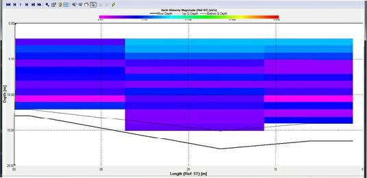
Figure 12: ADCP transect recorded at 13:54 UTC at the Carrick Roads sampling site shown on WinRiver.

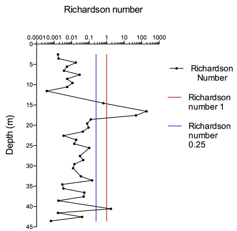
Figure 8: Richardson number fluctuations with depth (m) at the offshore sampling site during sampling.

Refer to Estuary page for explanation of the Richardson Number. The stations used were located further offshore than when collecting estuary data, such that flow was dominated by tides rather than riverine influx. Tides were as follows (taken from My Tide Times):

Measurements taken between 08:16 and 12:54 UTC were recorded during the ebb tide; data ascertained at 13:54 UTC represented the onset of low tide and all values  acquired from there onwards were part of the flood tide.

The 08:16 UTC CTD cast was taken offshore (figure 11); beyond the tidal front in stratified deep water. Observing the respective contour plot shows a thermocline, shown here by Richardson Numbers of above 1 at ~17m, indicating laminar flow. Well-mixed waters of the thermocline are surrounded either side by stratified waters. There is thus minimal change in flow velocity within the thermocline in relation to the stratified waters above and below it, such that laminar flow is present at the thermocline and turbulent waters either side.

Nonetheless, the majority of Richardson Numbers are below 0.25, indicating turbulent flow. In fact, the readings at 13:54 UTC are the only constituents of the time series in which no laminar flow was recorded. Riverine outflow from Carrick Roads is continuous, regardless of tidal state. Thus, at low tide, when movement of oceanic water masses is minimal, there is still movement of riverine water, even if very slow. The riverine water thus drags the stagnant oceanic water, hereby increasing shear. Although the absolute riverine flow is very small, the Richardson Number is a ratio such that the relative change in velocity with shear is of importance. As velocity change is minimal, but shear change quite large, this will result in small Richardson Numbers, i.e. turbulent flow.

From figures 8 and 9 it can be observed that flow throughout the ebb tide was mostly turbulent, but becoming more laminar at each station. Approaching low tide, the velocity of the ebb tide, and consequentially shear between the stagnant deeper water and motile surface water, decreases. This minimises turbulence.

Figure 10 shows the Richardson Number calculated from data collected at 13:54 UTC, which was taken at onset of low tide. One would expect low tide to result in least turbulent flow, yielding Richardson Numbers of above 1 (laminar flow). Indeed, when examining the velocity profile of the ADCP transect taken 13:54 UTC on WinRiver (figure 12), it can be observed that flow velocities are minimal.

The data recorded at 16:33 is the last of the time series, and closest to high tide (figure 11). The incoming tide potentially explains the turbulence shown by the low Richardson number in the surface water. The station is influenced by the outflowing river water at the top of the water column due to the low density. This is met by tidally driven sea water which increases mixing. This explains the overall low flow velocity with a high variability between layers; therefore causing a high degree of turbulence. At greater depths there are higher Richardson numbers, potentially due to less mixing of different water bodies. Therefore, there is less variability of flow velocity between depths, regardless of the higher flow speeds in relation to the shallower depths.