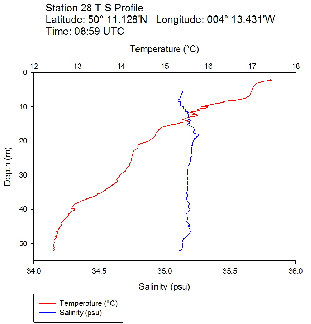
 Figure 38: Temperature salinity profile for station 28
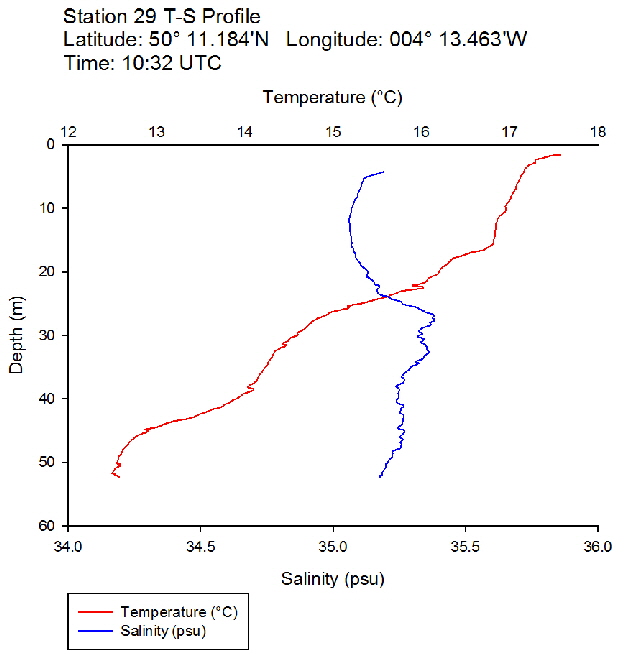 Figure 39: Temperature salinity profile for station 29
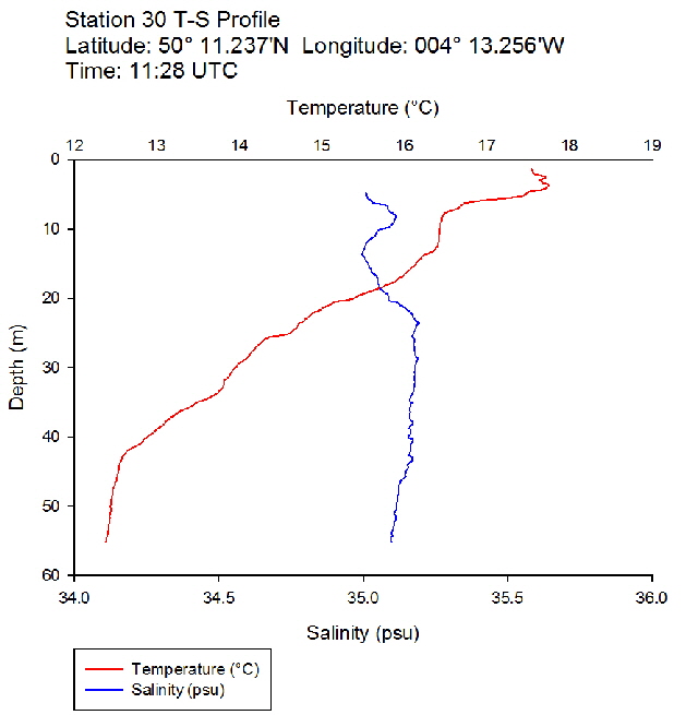 Figure 40: Temperature salinity profile for station 30
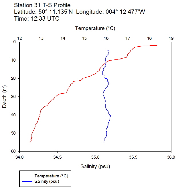 Figure 41: Temperature salinity profile for station 31
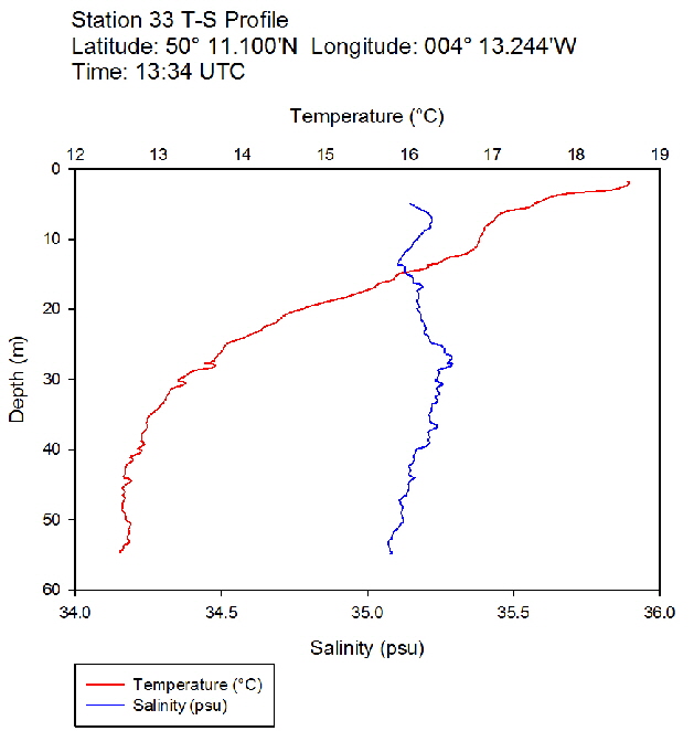 Figure 42: Temperature salinity profile for station 33
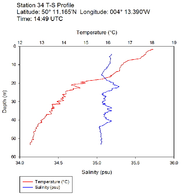 Figure 43: Temperature salinity profile for station 34
![]()
To understand the physical processes affecting the vertical structure of the water column in temperate, deep coastal waters, and how this affects phytoplankton and zooplankton vertical distributions in relation to irradiance and nutrient levels.

During the Summer, due to solar heating and weak surface currents and winds, the surface layers of temperate seas become stratified offshore. As the time series progressed throughout the day, the surface layer responded rapidly to the increase in solar radiation. The TS profiles (figures 38 to 43 ) show a clear diurnal warming on the surface layer throughout the time series. Figure 44 shows that warming of the surface layer was particularly prominent following midday where there was higher solar irradiance reaching the surface waters, increasing from a surface PAR of 790 Wm-2 at Station 28 (08.59 UTC) to 1112Wm-2 at Station 34 (14:49 UTC) (figures 51 to 55 ). The surface temperatures increased from 17.4°C at Station 28 (08:59 UTC) and reached a maximum of 18.6°C at Station 33 (13:34 UTC). The last station (Station 34 at 14:49 UTC) saw a decrease in the surface temperature back down to 18°C due to a change in weather conditions and sea state.
The TS profiles show a clear thermocline nearing the surface ranging at a depth of 10 – 20m across the time series, indicating a past mixing event. The deeper profiles follow a gentle thermocline to the seafloor, imitating the exponential decay of light from the surface and absent mixing. This is commonly seen in temperate offshore seas that have remained calm and unaffected by storm events over a period of time. As the weather had remained warm and very calm over the days prior to the data collection, this result is not surprising. The temperature profiles display a significant change with depth – the smallest change (5.0°C) observed at Station 28 (08:59 UTC) and the greatest (6.1°C) at Station 33 (13:34 UTC)

The fluorescence profiles (figure 45 to 50) were used as a proxy for chlorophyll, with an aim to identify the depth of the deep chlorophyll maximum and its movement across the time series. The deep chlorophyll maximum was seen to shoal from 10:32 UTC to 13:34 UTC, which could be indicative of diel migration of some phytoplankton species.
The depth of the maximum fluorescence also coincides with the minimum beam transmission. This indicates that the fluorescence maximum is at a depth where there is the greatest biomass of phytoplankton present. This is also shown by the phytoplankton cell counts, taken at appropriate depths in the water column. Phytoplankton samples from Station 29 (27m) and 30 (25.6m) were counted by one of the lab technicians, so this lead to unusual peaks in phytoplankton abundance as more cells can be identified with a professional eye. Station 28 (51.6m) contained an unusually large cluster of Cosconodiscus (estimated 132 cells) stuck to what looked like a gelatinous structure and lead to a result for this sample far higher than others at the same depth and may skew the results with a king kong effect.
The PAR profiles (figures 55 To 60) were used to indicate a rough estimate of the limit of photosynthesis (1% light level). The base of the euphotic zone was estimated at depths of 37m (Station 28), 41m (Station 29), 38m (Station 30), 35m (Station 31), 34m (Station 33) and 34m (Station 34). These depths correlate well with the fluorescence profile and show the cut off depth of photosynthesis with a decrease in fluorescence from the maximum paired with a decrease in phytoplankton abundance.
![]()
Station 32 (13:20 UTC) was used to yo-yo the CTD in attempt to visualise internal waves around 15 – 45m by looking at the movement of the fluorescence maximum (figure 56). The Brunt-Vaisala frequency was calculated to be 0.012s-1 with a period of 1.4 minutes. This period is seen clearly in cast 3 and 4 of the CTD (13:25:57 UTC – 13:27:31 UTC), showing the internal wave structure. With a short period, aliasing has occurred at points in the data set where the CTD missed the movement of the maximum fluorescence. Even so, a clear sinusoidal pattern of an internal wave structure can be seen.

To marry the proxy fluorescence with authentic chlorophyll values, Niskin bottles were fired at appropriate depths throughout the profile – above, at and below the maximum fluorescence on the CTD profiles. These chlorophyll values were graphed alongside the nutrient profiles (silicon, phosphate and total oxidised nitrogen (NO2 + NO3)) also collected in the Niskin bottles, to get an idea of the relationship. Calibration curves for fluorescence and chlorophyll were also created for further analysis. The nutrient values are low at the surface, indicative of uptake by phytoplankton in the euphotic zone. Beneath the deep chlorophyll maximum, nutrients begin to replenish, increasing at depth, which is evidence of remineralisation of dead phytoplankton sinking below the euphotic zone.
The concentration of silicon is limited in surface waters at every station – this can be explained by diatoms which use silicon in their tests. In the morning (Station 28), the silicon concentration remains low without fluctuating throughout the water column. As the day progresses, there is a peak of silicon concentration at around 20-30m – sampled at Station 30. At Station 34, the station latest in the day, the silicon concentration was highest at ~40m. This shows that throughout the day, the silicon abundance increases with time and depth.
The general trend seen on the graph for nitrate concentration shows that nitrate levels increase with depth – this trend was seen at each station. Station 28 and 30 show almost identical behaviour, peaking at ~50m with 1 µmol/litre nitrate concentration. In the samples taken in the afternoon, the change in nitrate concentration rises dramatically from 20–30m with a more than double increase in concentration.
Nitrite concentration increases with depth at each station. Stations 28, 30 and 33 all follow a relatively linear pathway, reaching concentrations of 0.1 µmol/litre at a depth of ~55m. However, Stations 29 and 31 show an unusually low concentration between the depths of 35-45m.
The graph which presents the total concentrations of Nitrates is similar to that of the nitrate concentration, where a gradual increase with depth has been displayed earlier in the day before a significant surge of total nitrates occurs at depths of around 20-30m in the afternoon. At the final Station, 34, there is an interesting plot line where the concentration rises sharply at two separate depths, the first occurring between 20-30m and the second between 40-50m.
Whilst analysing the depth profile for phosphate concentration, it is clear to see that the first 5 Stations (28-33) follow a very similar trend where levels remain low at surface waters rising gradually with depth until they peak at a concentration of 0.2 µmol/litre and 55m depth. However, Station 34 presents an intriguing pattern where concentrations decrease significantly with depth. Surface waters experiencing concentrations of around 0.34 µmol/litre which is followed by a sudden drop to 0.03 µmol/litre at 20m, until it increases slowly to 0.2 µmol/litre where it overlaps with the data displayed from other Stations.

Abundance :
The abundance of phytoplankton found at each depth for Station 28 to 34 is presented in figure 62 When making comparisons between our abundance and diversity data (figure 63), it is interesting to see how Station 28, which has the highest abundance, has the lowest diversity of species. The intentions of creating a time series was to enable us to witness diurnal migration of phytoplankton across a number of hours, this can be detected in this graph. The abundance of organisms found at surface waters is minimal in the early morning, whilst sampling at station 28 at 08:58:00 UTC, however the abundance is very high in deeper waters at this time. As we progress through the day, moving along to the right of the graph we can see a gradual increase in the number of organims being found in surface waters and decreasing numbers found in deeper waters. Another intriguing correlation between the graphs of diversity and abundance would be that, on a whole, the highest numbers of both variables were found between 25-35m depth.
Diversity:
The diversity of phytoplankton species at each station is displayed in figure 63 This was calculated using the total number of individuals found at each depth, separated into stations by colour. Depth was chosen as the X variable because time only differs by a small amount within each station, this also enables us to make comparisons with the data obtained on the chlorophyll maximum depths. The data presented was obtained from a time series, therefore the location at each station remained the same, with time as the variable across stations. Sampling at Station 30 began at 11:28:00 UTC and this shows the largest amount of diversity between species of phytoplankton. In addition to this, the diversity is typically highest between depths of 25-35m.

A clear temporal variation in the vertical distribution of zooplankton was observed throughout the day, indicating a dial migration, possibly coordinated with that of phytoplankton. 10 mL of water were analysed at each station.
At 9:00 in the morning, the highest abundance of zooplankton was found in the surface layer between 0 and 12 m depth, with a species abundance approaching 50 cells per. Zooplankton was still relatively abundant at depth at this time, exceeding 30 cells between 30 and 40 m depth. Abundance between 5 and 15 m depth remained similar at 10:32 to that measure at 9:00, but abundance in the bottom layers between 35 and 45 m depth fell to about 5 cells. Abundance increased in the surface layers at 11:28, peaking at about 55 cells, while increasing again in the 30-40 m depth section to reach approximately 32cells. Zooplankton abundance increased to more than fifty at the same depth at 12:33, but fell again to about 5 cells at 13:34. Abundance between 10 and 20 m depth remained above 50 at 13:34, but was approximately divided by two at 14:49. Zooplankton abundance was then above 50 cells between 35 and 45 m depth by 14:49.
Zooplankton species abundance (Callista)
Ten mL of water were analysed for every station.
Globally, the most abundant zooplankton genus present in samples throughout the day was Copepoda, with relatively similar abundances at all stations (about 15 cells), except for station 30 and station 34 which had copepod abundances of respectively about 27 and 24.
Cladocera were also abundant over at all stations, except station 29 where abundance was less than 5 cells counted.
Echinoderm larvae were under 20 cells except for station 30, where more than 30 cells were counted.
Less than 5 Copepod nauplii, Polychaete larvae, Tunicate, Bryozoa, Appendicularia, Siphonophore, Chaetognath and Decapod larvae cells were counted for each station.
Hydromedusae larvae had an abundance inferior to 5 cells across all stations except stations 28 and 29 where they respectively about 5 and 9 cells were counted.

On 7th July 2018, Callista took group 8 offshore to Station 28 (Latitude: 50° 11.128’N, Longitude: 004° 12.431’W), located in deep water (56m) off the coast of Plymouth, east of Eddystone Rocks. We stayed on station for most of the day, carrying out CTD measurements every hour to conduct a time series of the various parameters of the water column such as temperature, salinity, fluorescence and PAR. Niskin bottles were used at appropriate depths to collect samples to process in the lab for chlorophyll, oxygen, nutrients and phytoplankton. A plankton net was also deployed to appropriate depths to sample for zooplankton. The conditions were optimal, with a particularly calm sea, barely any wind and not a cloud in the sky. The time series correspond to Stations 28, 29, 30, 31, 33 and 34 accordingly. Station 32 was used to yo-yo the CTD in the water column between depths of 15 and 45m to attempt to visualise internal waves by a sinusoidal movement of the maximum fluorescence.
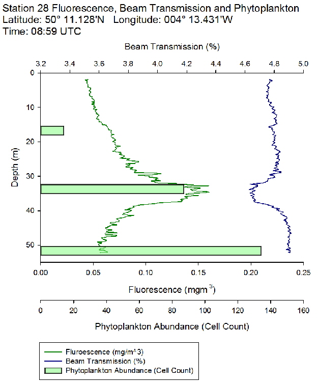 Figure 45: Fluorescence, beam transmission and phytoplankton count for station 28
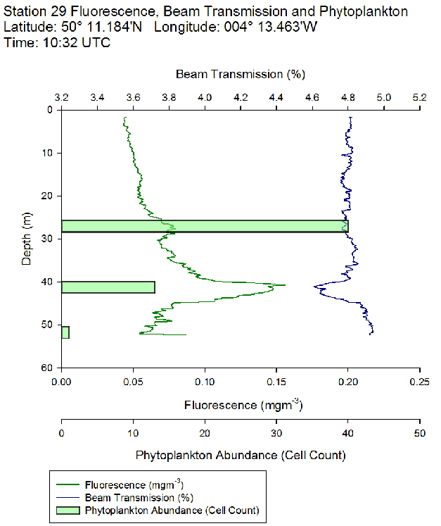 Figure 46: Fluorescence, beam transmission and phytoplankton count for station 29
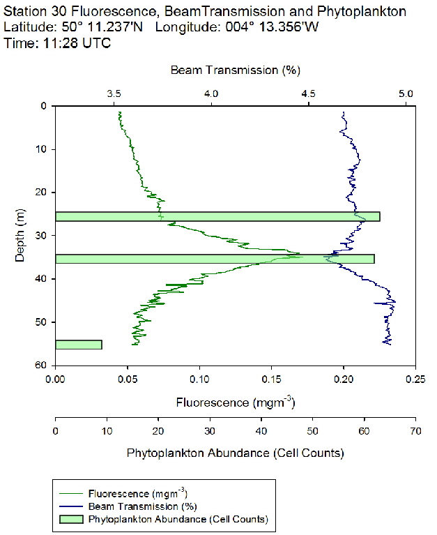 Figure 47: Fluorescence, beam transmission and phytoplankton count for station 30
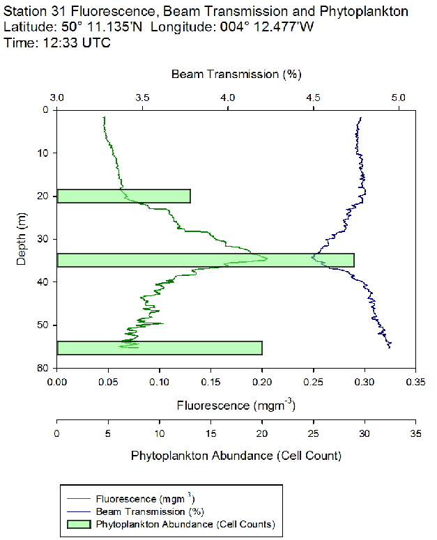 Figure 48: Fluorescence, beam transmission and phytoplankton count for station 31
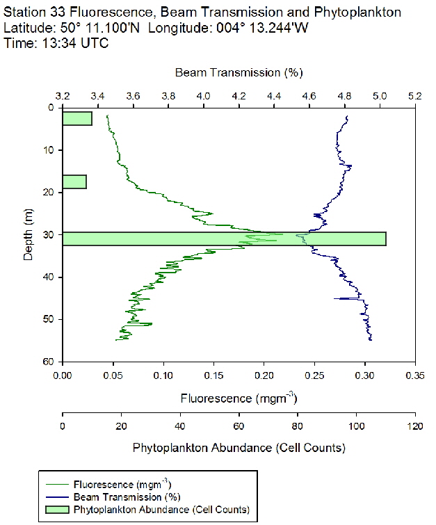 Figure 49: Fluorescence, beam transmission and phytoplankton count for station 33
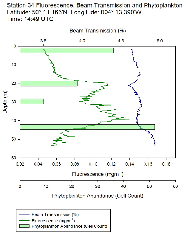 Figure 50: Fluorescence, beam transmission and phytoplankton count for station 34
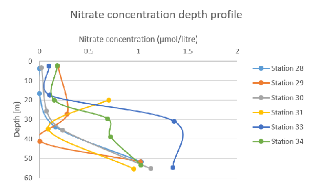 Figure 57: Nitrate concentration depth profile for all stations
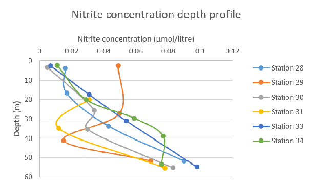 Figure 58: Nitrite concentration depth profile for all stations
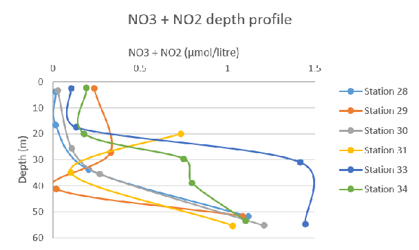 Figure 59: Total nitrogen species concentration depth profile for all stations
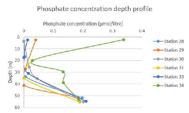 Figure 60: Phosphate concentration depth profile for all stations
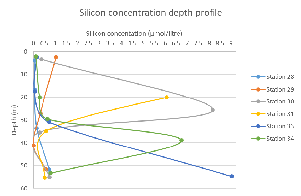 Figure 61: Silicon concentration depth profile for all stations
![]()
A CTD was deployed up and down the water column every hour at approximately the same location. Water samples were taken near the seabed, at the deep chlorophyll maximum and at the bottom of the thermocline using Niskin bottles attached to the rosette .Phytoplankton Samples were preserved using lugols Iodine.
A zooplankton closing net was then deployed to sample depths of high Chlorophyll concentrations detected by the CTD.


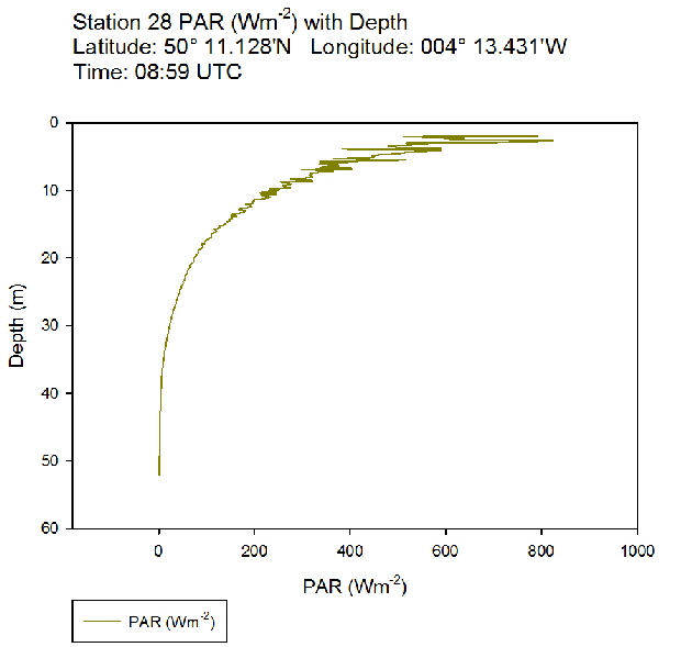 Figure 51: PAR profile for station 28
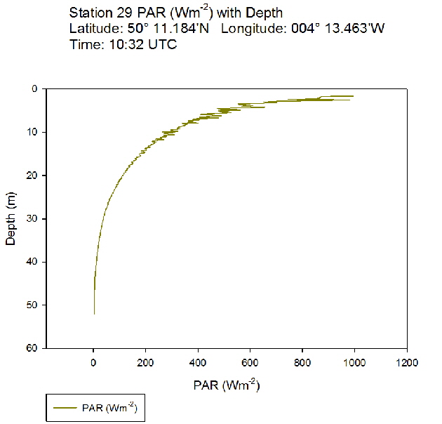 Figure 52: PAR profile for station 29
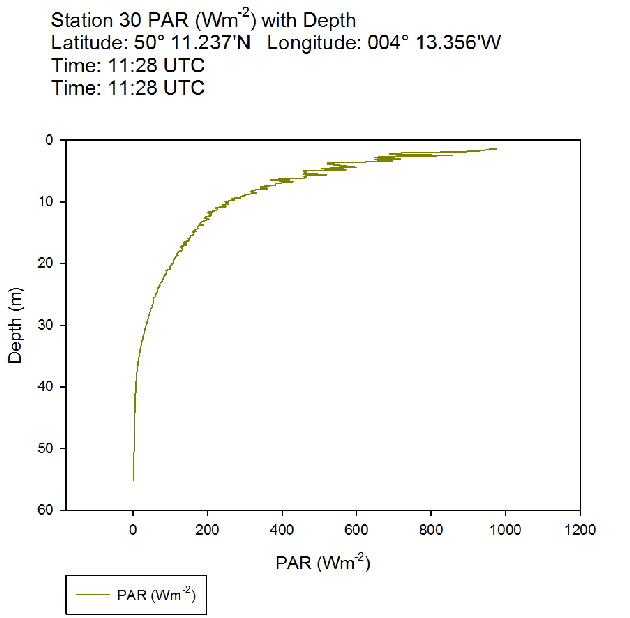 Figure 53: PAR profile for station 30
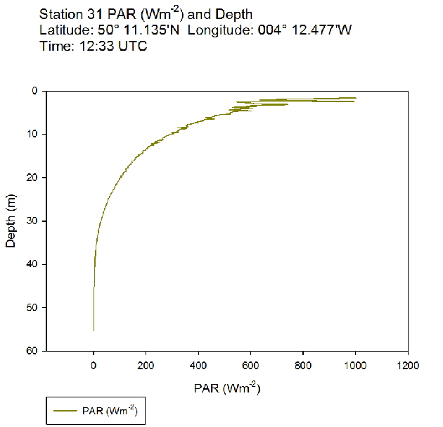 Figure 54: PAR profile for station 31
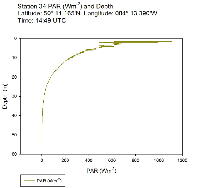 Figure 55: PAR profile for station 34
Figure 56: Depth of maximum fluorescence (deep chlorophyll maximum)
Figure 62: Offshore phytoplankton abundance for all stations
Figure 63: Offshore phytoplankton diversity for all stations
Figure 64: Offshore Zooplankton abundance for all stations
Figure 65: Offshore zooplankton diversity for all stations
PLYMOUTH FIELD COURSE: THE INITIAL FINDINGS OF GROUP 8