

Disclaimer: The views expressed in this website are not those of the University of Southampton or the National Oceanography Centre

Offshore

Contents
Information
Date: 27/06/15
Vessel: R.V. Callista
Weather: Fair. No measurable precipitation
Sea State: Small waves, frequent white horses.
Cloud Cover: 3/8
Tide: Low tide (1.70m): 8:18 UTC
High tide (4.20m) 14.17 UTC
Location: 50°05.67’N, 4°52.02’W
8:36 UTC – beginning of ebb tide going out. Weak tidal flow at this time, westerly flow out to the channel.
Profile 1
Lat: 50˚05.543N
Long: 004˚52.011W
Time UTC: 8:05:29
Profile 2
Lat: 50˚05.529N
Long: 004˚51.330W
Time UTC: 8:48:15
Profile 3
Lat: 50˚05.708N
Long: 004°52.115W
Time UTC: 9:24:00
Zooplankton net samples:
1st net depth: 45m-
Time UTC: 9:57:25 – 9:58:04
2nd net depth: 35m-
Time UTC: 10:13:03 – 10:13:15
3rd net depth: 25m-
Time UTC: 10:24:32 – 10:26:10
Profile 4
Lat: 50°05.660N
Long: 004°52.014W
Time UTC: 10:33:30
Profile 5
Lat: 50°05.616N
Long: 004°52.115W
Time UTC: 11:00:00
In the first week of Falmouth, all the offshore sampling expeditions had collected samples from a widespread group of stations, with all groups collecting samples from ‘the standard station’ also known as station B. For this trip offshore, the decision was made to compile a time series data set of station B, in order to look at how the physical factors at this station changed during the day, giving the other stations a set of data to compare to. Also, the time series would demonstrate how factors like plankton abundance, temperature, fluorescence and irradiance change throughout the day, possibly due to the altering wave action, tides and weather.
Conditions
South westerly prevailing winds with a large fetch blowing across the Atlantic make offshore at Falmouth an exposed area.
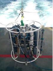
5 profiles were made at Station B using the CTD rosette (figure 1):
The rosette contained a number of devices of which only 6 Niskin bottles and the CTD itself were used.
At each station the rosette was sent down to c.60m and returned to the surface, measuring a number of parameters, mainly noting temperature, fluorescence and irradiance.
At profiles 1, 3 and 5 Niskin bottles were fired at different depths. Once the CTD reached the bottom of the profile, the dry lab team decided the most effective depth to sample and on the return to the surface fired the Niskin bottles at these chosen depths.
From the Niskin bottles, water samples were taken:
- 1 sample per depth was taken in a glass bottle immediately after the Niskin bottle was opened, for measuring dissolved oxygen. Two reagents were added to the sample to form a precipitate to prevent the oxygen leaving the sample before processing in the lab. One sample per depth was taken for silica, stored in a plastic bottle to prevent the silica being scavenged before processing.
- 1 sample per depth was for nitrate and phosphate, stored in a glass bottle. Plastic is capable of scavenging phosphate out of samples (although very slowly).
- 3 samples per depth were taken for chlorophyll. The water samples were passed through a filter by syringe and the filter was then stored in acetone for later processing.
- Phytoplankton samples were taken from the Niskin bottle by collecting them on a filter while pushing them through a syringe.
- Additionally, measurements for fluorescence, salinity and temperature were recorded from the CTD at the firing depths, to complement the sampled data.
Figure 1 -
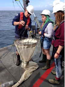
Figure 2 -
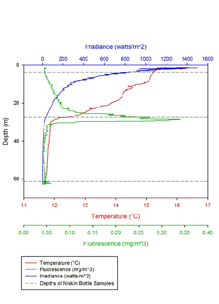
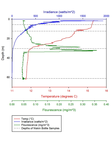
Figure 3 -
Figure 4 -
The graphs clearly show the thermocline and how it alters throughout the day. The thermocline is where the highest abundances of plankton are seen, due to the action of mixing both above and below it. The fluorescence peak indicates the highest peak of plankton and therefore reveals the position of the thermocline. The profiles demonstrate that levels stay relatively constant throughout the day, except for some minor temperature changes. The only significant change is that in the last profile, the irradiance level begins at 4000, when the other stations show numbers closer to 2000, or below. This is likely due to a few contributing factors, for example that profile 5 was taken later in the morning when the sun was higher in the sky and also as the morning carried on, cloud cover decreased, which would increase irradiance. In general, however, these profiles are very similar, demonstrating that station B, as the standard station didn’t alter much throughout the day and any changes would most likely be long term. This makes station B a good standard to compare the other stations.
Thermoclines are areas of rapid change in temperature. They are formed when the surface
layer of a body of water is heated up, making it less dense, whilst the water below
remains cool. The thermocline at station B is broken up into two parts (figure 6).
The double thermocline may be due to a small amount of mixing within the surface
layer. At 8-
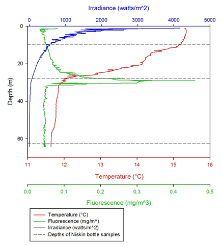
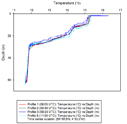
Figure 5 -
Figure 6 -
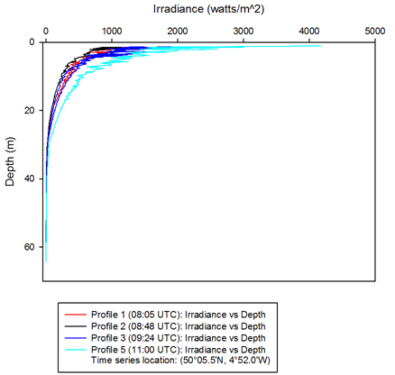
Irradiance decreased exponentially with depth in water due to light being scattered
and reflected by particles and water molecules (1). Light penetrated to a greater
depth as time progressed in the day due to an increase in solar radiation (figure
7). Photosynthesis can occur at 1% of the surface light. Surface irradiance values
for most of the time points were between 1500-
Left: Figure 7 -
Below: Figure 8 -
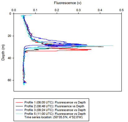
The depth of the chlorophyll maxima in the water column is indicated by the large
peaks seen in the fluorometry-
Fluorescence slowly increased from 0.04 v at the surface, to 0.09 v at around 20
m during the three hours of sampling at station B (50°05.5'N, 4°52.0'W). Fluorescence
peaked between 25 m and 33 m at each time the water column was sampled. At 08:05
UTC there was a double peak of fluorescence, with the first peak being at a similar
depth to the other time profiles (~28 m) and the second peak being at around 32-
Samples were chemically analysed via the same methods used for processing estuarine samples.
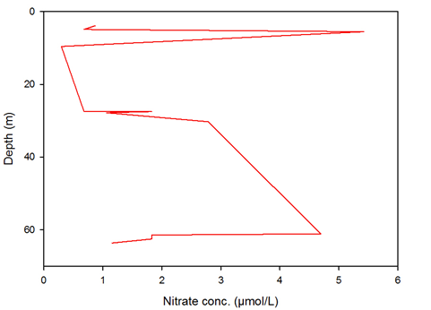
Nitrate concentration is clearly depleted, beginning at around 10m and stays at a low level until it approaches 30m where it begins to increase in concentration until c.60m where it is again reduced. This depletion below the surface waters is result of the thermocline, where the highest abundance of plankton is found, and therefore almost all available nitrate is used up for growth. Below the thermocline, c. late 20s/low 30metres, the mixing in the water column nutrients from depth, causing an increase in nitrate concentration. The depletion at the seafloor (c.60m) is likely due to benthic organisms’ nutrient intake.
Figure 10 -
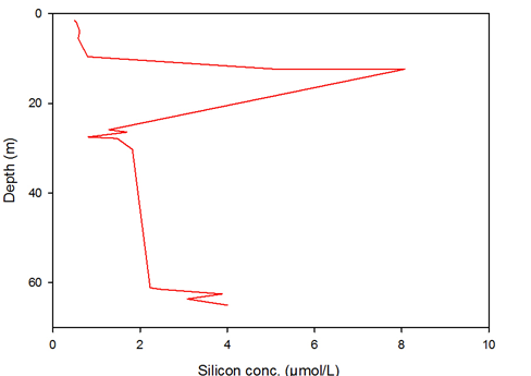
Figure 11 -
Silicon concentration is increased quickly just below the surface due to mixing until it reaches around 10m. From then on a severe trough is seen, demonstrating depletion by organisms, predominantly diatoms above and in the thermocline, where they are most abundant. Below the thermocline, the concentration slowly increases, but not to the same concentration seen before the thermocline. The heightened increase at the seabed is due to dead diatom bodies reaching the seabed and dissolving to release silicon again into the water column.
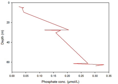
Figure 12 -
Phosphate shows a small depletion at c.28m, in the centre of the thermocline; however on the whole it slowly increases in concentration down the water column. This is most likely due to the fact that phosphate is present in such low concentrations that after being depleted at the thermocline, it takes little time for the concentration to be replenished by mixing.
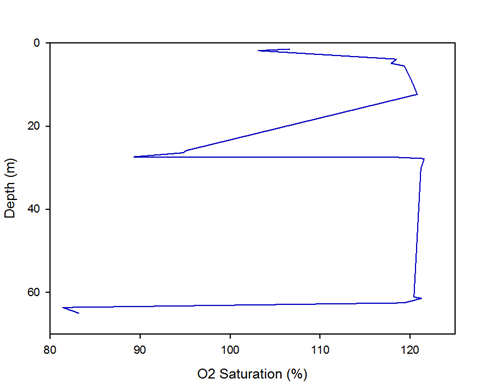
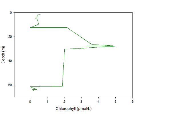
Figure 13 -
The distribution is similar to the distribution of nitrate, with saturation through the water column is relatively constant apart from the depletion shown from 10 to 30metres and depletion at the seabed, c. 65m. The trough is due to the highest abundance of plankton (and therefore bigger animals) in and above the thermocline, causing an increase in O2 demand and hence a depletion in O2 saturation. The decrease in saturation at the sea bed is (again similar to nitrate) due to benthic organisms.
Chlorophyll follows a similar distribution to silicon, although the main part of the peak is a little lower, at c.30m, almost the centre of the thermocline. After the thermocline, the chlorophyll, expectedly, decreases until the bottom of the sea bed as less light is available and photosynthesis becomes impossible.
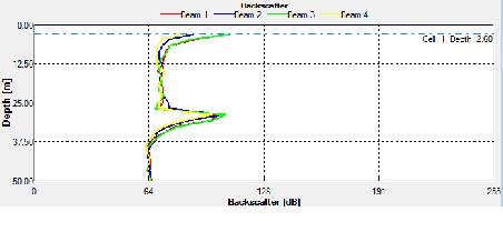
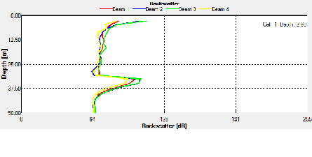
ADCP Offshore data
ADCP data was taken for the entire time series at station B from 0801-
Figure 9 -
Figure 14 -
- Lorenzen, C. (1972) Extinction of Light in the Ocean by Phytoplankton. ICES Journal
of Marine Science, Volume 34, Issue 2, pp. 262-
267 - Spector, D. (1984). Dinoflagellates. Orlando: Academic Press.
- Ichimi, K., Kawamura, T., Yamamoto, A., Tada, K. and Harrison, P. (2012). Extremely
High Growth Rate of the Small Diatom Chaetoceros salsugineum Isolated from an Estuary
in the Eastern Seto Inland Sea, Japan 1. Journal of Phycology, 48(5), pp.1284-
1288. - Steele, J. (1978). Spatial pattern in plankton communities. New York: Plenum Press.
- Ianora, Adrianna, Serge A. Poulet, and Antonio Miralto. 'The Effects Of Diatoms On
Copepod Reproduction: A Review'. Phycologia 42.4 (2003): 351-
363. - De Bernardi, R et al. (1978). Cladocera; Predators and Prey. Developments in Hydrobiology
35 225-
243 - Vergara-
Soto, Odette et al. 'Functional Response Of Sagitta Setosa (Chaetognatha) And Mnemiopsis Leidyi (Ctenophora) Under Variable Food Concentration In The Gullmar Fjord, Sweden'. Revista de biología marina y oceanografía 45.1 (2010)
Phytoplankton
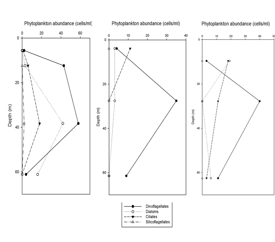
Dinoflagellates were the most abundant phytoplankton throughout the time series taken at this station. This is to be expected, as dinoflagellates bloom after the diatom spring bloom when nutrient levels are lower and there is less competition with the larger diatoms (2). Throughout the entire time series dinoflagellates greatly exceeded any other phytoplankton group, with the total number being 209 cells/ml whilst diatoms were only found at 92 cells/ml.
Interestingly, it can be seen that the majority of the dinoflagellate population
maintains a fairly stable position in the water column, around 30-
Zooplankton
Throughout the time series experiment on Callista three Zooplankton closing net transects
were taken consecutively, between 0-
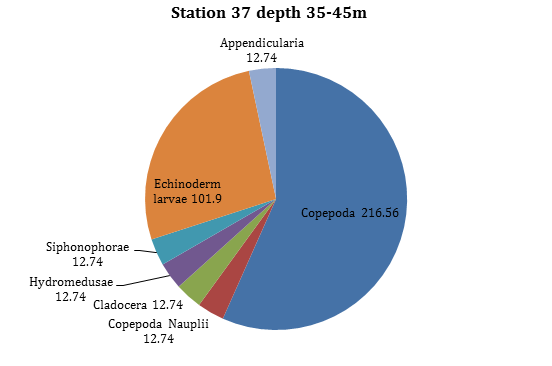
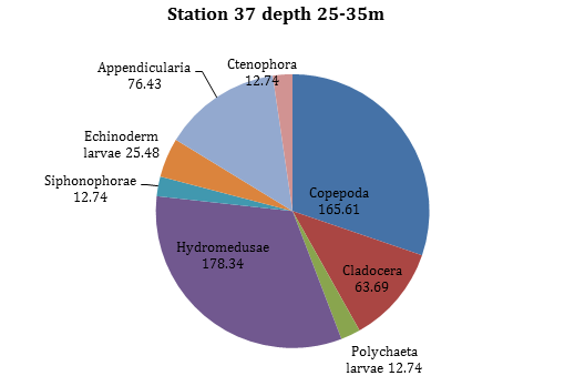
Figure 18 -
Figure 19 -
Copepoda, Cladocera, Hydromedusae and Echinoderm larvae are the most prolific, whilst other species were recorded in much smaller concentrations. There is a thermocline at 10m and 35m. The Dinoflagellates are the most abundant around the thermocline with other phytoplankton migrating into greater light intensities diurnally. A diverse phytoplankton community will support a healthier zooplankton community. Copepoda increase in abundance with depth, and they are at there greatest concentration around the thermocline.
Both Copepoda and Echinoderm larvae are most prolific at this depth (between 35-
In the middle of the water column between 25m-
At the surface between 0-
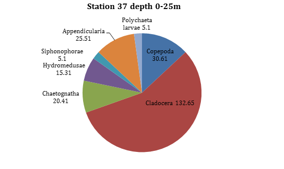
Figure 20 -
Start time -
Start time -
Start time -
Figure 15 -
Figure 16 -
Figure 17 -
Between profiles 3 and 4, three closing nets were used to collect samples of the
zooplankton present in the water column. A weighted closing net was used, which was
deployed to a decided depth eg. 45m and then pulled up to a shallower depth, eg.
35m. A messenger was then deployed to close the net, creating a sample of a section
of the water column. The 3 trawls carried out were from 45-