

Disclaimer: The views expressed in this website are not those of the University of Southampton or the National Oceanography Centre
Geophysics
Date: 25/06/2015
Vessel: RV Explorer
Weather: Fair – no significant precipitation
Sea State: smooth
Cloud Cover: 3/8
Tides: High tide (4.10m) at 11:05 UTC.
Low tide (1.8m) at 17:35 UTC.
Departed: 11:45 UTC
Transect 1 (Ken 005)
Start time: 13:34:32 UTC
Start Location: 50°06.0N 005°07.0W
End Time: 13:38:07 UTC
End Location: 50°06.0N 005°06.6W
Transect 2 (Ken 004)
Start Time: 13:42:58 UTC
Start Location: 50°06.0N 005°06.6W
End Time: 13:46:37 UTC
End Location: 50°06.0N 005°07.0W
Video 1
Start Time: 14:03 UTC
Start Location: N 26374.0m, E 177265.8m
End Time: 14:20 UTC
End Location: N 26971.0m, E 177139.1m
Video 2
Start Time: 14:28 UTC
Start Location: N 271546m, E 177723.9m
End Time: 14:45 UTC
End Location: N 27115.5m. E 177686.2m

Contents
Information
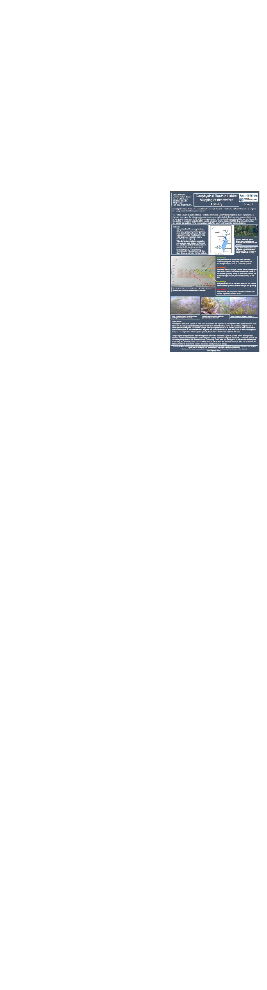
The Helford river estuary has been designated as a marine special area of consideration (SAC). This status was given due to its rich and varied ecosystems including maerl and eelgrass beds.
Aim:
To investigate the benthic seafloor within the Helford Estuary and map the geological and biological features of this area. Particular interest was given to the artificially planted eelgrass by Dr. Ken Collins.
Objective:
To use the side scan sonar to create a benthic habitat map and thus map the eelgrass and then use a drop camera to ground truth our findings.
A survey of the Helford lower estuary was conducted using a sidescan towfish and a live video feed to determine the bathymetric features.
Fal and Lower Helford is a Special Area of Consideration, it has numerous habitats that are rare and fragile (1). These include the Maerl beds, most abundant at the St. Mawes bank, which is in fact one of the UK’s only and largest maerl beds (2). The Helford Estuary, a part of the Falmouth Bay, is an idyllic location, with many boats moored along the edges and small beaches, this however is detrimental to the existence of the delicate eelgrass beds that lie near the banks of the Helford.
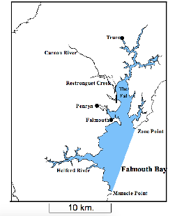
Figure 1 -
Eelgrass
Eelgrass (Zostera spp), is one of the few angiosperms that permanently inhabits submerged
marine environments. Human-
Figure 2 -
Figure 3 -
Sidescan Transect
Once the area of interest had been located-
Video transects
Two transects were taken, one across the side scanned area, footage of the MCZ was also taken. This can be used to identify species present and percentage cover of the eelgrass.
Using the programme ImageJ a ratio was calculated that compared the two most dominant species in both transects algae and seagrass. This was done by selecting a number of frames throughout the video, in each of these frame using a free hand lasso tool a species was drawn around and the pixels in the area selected allow a percentage cover of the species to be generated.
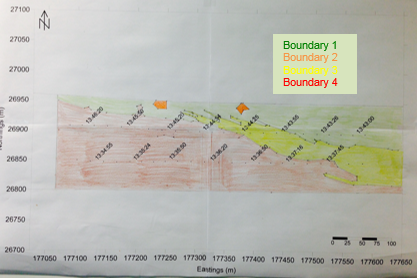
Habitat Map
The habitat map was created by preliminarily aligning the two scan print outs and
combining them to create one image of the survey area. Using time and position a
skeleton was constructed on the programme Surfer, the time could cross-
Findings from the final profile were classified by the knowledge of sediment reflectivity and then comparing to the video feeds. The less reflective the sediment, the softer the benthos, this then indicates softer sediments. The sediments towards the bottom of the habitat in boundary 4 are hard since they produced greater backscatter. The eelgrass however produced more backscatter, this paired with the video footage showed the areas where these eelgrass communities were present.
Seagrasses are generally known as ecosystem engineers, as they reduce flow velocities in their canopies. In perennial subtidals they usually lead to increased net sedimentation rates and reduction of the grain size (4). This could explain why sediment seems appears to be a harder substrate on the benthic habitat map.
Left: Figure 6 -
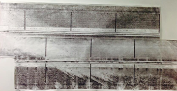
Figure 5 -
Analysing and comparing the video footage of the two different areas allows a comparison
between a well-
Transect 1 had both a side scan sonar and video footage to record the bathymetry. This transect covered the area where the seagrass was implanted.
Transect 2 had just a video recording of the benthos. The bedform and biota was monitored
in this area since it is a Marine Conservation Zone that acts as a well-
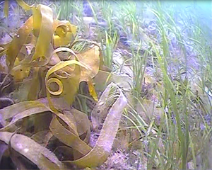
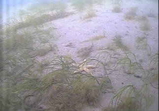
Right: Figure 7 -
These two images (figures 6 and 7) are from each of the video footage transects.
A clear difference can be seen between transect 1, in image 3 and transect 2, in
image 2. There is a much greater density of seagrass and other macroalgal species
in image 2 in the well-
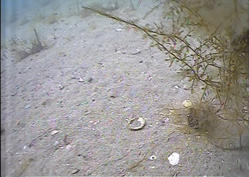
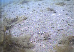
Figure 8 -
Figure 9 -
|
Time (in video) |
Type |
Total area (pixels) |
Seagrass /algae |
|
Transect 1 |
|||
|
02:00 |
Seagrass |
7062 |
0.04 |
|
|
Algae |
175093 |
|
|
04:00 |
Seagrass |
27768 |
0.12 |
|
|
Algae |
233848 |
|
|
06:00 |
Seagrass |
3176 |
0.01 |
|
|
Algae |
304839 |
|
|
08:00 |
Seagrass |
13397 |
0.37 |
|
|
Algae |
35787 |
|
|
10:00 |
Seagrass |
570945 |
3.39 |
|
|
Algae |
168455 |
|
|
Transect 2 |
|||
|
02:00 |
Seagrass |
14972 |
0.04 |
|
|
Algae |
336127 |
|
|
04:00 |
Seagrass |
22483 |
0.05 |
|
|
Algae |
439001 |
|
|
06:00 |
Seagrass |
3795 |
0.02 |
|
|
Algae |
181495 |
|
Table 1 -
The density of seagrass was greater in the natural habitat as seen in the video footage,
however on analysis of the ratio between seagrass and algae Transect 1 had higher
ratios of Seagrass to Algae whereas transect 2 has less seagrass to algae. There
is a similar abundance of eelgrass seen in both transects however it is unknown how
much is the implanted biota. The success can also be judged upon the health of the
surrounding community. Hardly any Laminaria species were identified in transect 1
whereas in transect 2 much of the eelgrass was flowering and there were algal pockets
as well as more shoals of juvenile fish can be seen. This could mean that the gradient-
- Langston, W.J., Chesman, N.C., Burt, G.R., Hawkins, S.J., Readman, J. and Worsfeild,
P. 2003, ‘Site Characterisation of the South West European Marine Sites-
Fal and Helford cSAC’, Marine Biological Association Occasional Publication No. 8. - Birkett, D.A., C.A.Maggs, M.J.Dring. 1998. Maerl (volume V). An overview of dynamic and sensitivity characteristics for conservation management of marine SACs. Scottish Association for Marine Science. (UK Marine SACs Project). 116 page
- Kemp WM, Twilley RR, Stevenson JC, Boynton WR, Means JC (1983) The decline of submerged vascular plants in upper Chesapeake Bay: Summary of results concerning possible causes. Mar Technol Soc J 17:78–89
- Bos, A., Bouma, T., de Kort, G. and van Katwijk, M. (2007). Ecosystem engineering
by annual intertidal seagrass beds: Sediment accretion and modification. Estuarine,
Coastal and Shelf Science, 74(1-
2), pp.344- 348. - Bouma, T.J., et al., 2005. Trade-
offs related to ecosystem engineering: a case study on stiffness of emerging macrophytes. Ecology, 86,2187-2199 - JNCC, 2011.Intertidal sediments dominated by aquatic angiosperms. [Online]
Available at: http://jncc.defra.gov.uk/page-5793
[Accessed 30/06/15]. - Tyler-
Walters, Dr. H., 2008. Zostera marina. Common eelgrass. Marine Life Information Network: Biology and Sensitivity Key Information Sub- programme [Online].
Available at: http://www.marlin.ac.uk/generalbiology.php?speciesID=4600
[Accessed 28/06/15]. - Pickett, S. (1976). Succession: An Evolutionary Interpretation. The American Naturalist, 110(971), p.107.
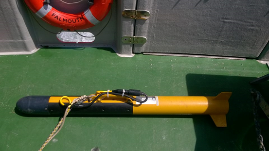
Figure 10 -
Figure 4 -