

Disclaimer: The views expressed in this website are not those of the University of Southampton or the National Oceanography Centre

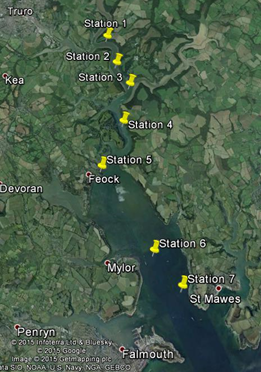
Sampling was carried out on the Bill Conway starting upstream at station 1 moving downstream to station 7 at Black Rock, located at the mouth of the estuary.
At each station a vertical CTD profile was taken. An ADCP transect was taken at station
1 only due to an equipment fault. A full set of ADCP data would have enabled us to
calculate the Richardson number at each station to compare flow stability moving
down the estuary. At stations 1, 2, 6 and 7 two Niskin bottle samples were taken
and at stations 3-5 three samples were taken. The depths were selected at each station
using the CTD profiles. Chlorophyll and nutrient (nitrate, phosphate and silicon)
samples were taken from every depth.
Less repeats and depths were sampled for dissolved oxygen and phytoplankton due to a limited number of storage bottles available. Dissolved oxygen was only sampled at the surface and bottom depth. Phytoplankton samples were taken from the surface at stations 1, 2, 4 and 7 only. Repeats were taken for each variable except chlorophyll. Zooplankton trawls were taken from stations 1, 3 and 7 using a 1m diameter net. Length of the trawls were measured using a flowmeter. Preservatives were added to plankton samples.
At each station a Secchi disc was used to estimate the depth of light penetration. From this the depth of the euphotic zone was calculated.
(Back to top)
Estuary
Date: 22/06/2015
Vessel: RV Bill Conway
Tide: High tide: 8:40 UTC (4.5m)
Low tide: 15:14 UTC (1.3m)
Weather
Cloud cover: 8/8
Wind: 2 (beaufort scale)
Station 1
Location: 50˚14.391N 005˚00.879W
Time: 11:57 UTC
Station 2
Location: 50˚13.731N 005˚00.947W
Time: 13:13 UTC
Station 3
Location: 50˚13.325N 005˚01.605W
Time: 13:54 UTC
Station 4
Location: 50˚12.548N 005˚01.618W
Time: 14:34 UTC
Station 5
Location: 50˚12.144N 005˚02.427W
Time: 15:08 UTC
Station 6
Location: 50˚10.276N 005˚02.143W
Time: 15:38 UTC
Station 7
Location: 50˚08.836N 005˚01.536W
Time: 16:04 UTC
River end members located in the Truro River.
The Fal estuary extends from its entrance between Pendennis Head and St Antony Head to its northernmost tidal limit at Tresillian. The estuary has a small riverine input and large tides which results in temperature and salinity differences throughout the estuary. The estuary is subject to natural and anthropogenic inputs which effects nutrient and biological distributions.
Aim:
To investigate how biological, chemical and physical properties vary throughout the Fal estuary as well as vertically at each station.
Objectives:
Determine physical properties including temperature, salinity, attenuation coefficient and turbidity.
Determine biological changes focusing on phytoplankton, zooplankton and chlorophyll.
Measure chemical changes including nitrate, phosphate, dissolved silicon and dissolved oxygen.
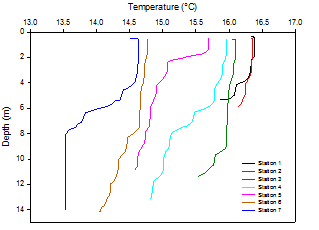
Temperature
Moving down the estuary temperature decreases throughout the water column. A decrease
of 1.4°C was observed in surface waters between stations 1 and 7 (Figure 1). Temperatures
are lower further downstream because of tidal dominance. In the upper estuary (stations
1-3) temperature varied little with depth. This is due to mixing throughout the water
column because the riverine and tidal inputs are interacting. Figure 2 shows that
from station 4 onwards temperature increases significantly with depth. The increase
was gradual for stations 4 and 6 whereas a thermocline was observed at stations 5
and 7. Reduced mixing results in the surface waters being heated. Cooler, denser
waters lied below. For example at station 7 surface temperatures were 1.1°C higher
than at 8m. Stations without an obvious thermocline show partial mixing between surface
and underlying water column.
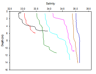
Salinity
Figure 3 shows that surface salinity increases by 2.2 from 32.8 at station 1 to 35.0
at station 7. In the upper estuary river inputs have a greater impact whereas in
the lower estuary seawater dominates. At station 1 salinity varies significantly
with depth from 32.8 at the surface to 33.9 at 5.3m. This is due to less dense riverine
water lying above denser saline water. At all stations, salinity increases with depth,
however increases are more noticeable in the upper estuary. Stations 6 and 7 show
very little salinity variation with depth. The salinities close to 35 at these stations
implies little to no influence of riverine inputs. The middle part of the estuary
(stations 3-5) shows small riverine influence in surface waters which is why salinities
are lower than at depth. The gentle gradient shows partial mixing in this area. In
general, salinity at all stations is shown to be quite high (figure 3) showing the
dominance of tidal input over riverine input in the Fal estuary.
Secchi Disc
Table 1 shows that the secchi disc depth increases with movement down the estuary and therefore the euphotic zone depth also increases. Euphotic zone depth increases from 6.6m at station 1 to 18.0m at station 7. The decrease in attenuation coefficient (k) reflects this trend. At stations lower down the estuary where the euphotic zone is deeper less light is attenuated by the water column. The value k is an indication of the amount of organic and inorganic particles in the water column which scatter light and so is linked to turbidity.
It is important to take into account limitations of this method as the line must be kept vertical, the disc must remain horizontal and there is the risk for human error. Therefore these results are estimations only
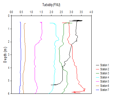
Turbidity
Figure 2 demonstrates that surface turbidity decreases as you move from station 1 at 3.11 FNU to station 7 at 0.43 FNU. Turbidity is highest at station 1 because of sediment input via rivers resulting in high levels of suspended particulate matter and lowest at station 7 because of little riverine influence.
At each station, turbidity varies little with depth except at station 1 where the
deepest reading is 1.11 FNU lower than the surface reading with a steady decrease
in turbidity occurring between the two points. Turbidity may vary with depth at station
1 as this is where the turbidity maximum occurs. The turbidity maximum responds to
changes in river flow1, largely influencing the turbidity of the surface waters.
When river flow increases, increasing stratification gradually decouples the upper
and low water layers so that an increasing proportion of the river-
|
Station |
Secchi disc depth (m) |
k |
Euphotic zone (m) |
|
1 |
2.2 |
0.654 |
6.6 |
|
2 |
2.5 |
0.576 |
7.5 |
|
3 |
2.7 |
0.533 |
8.1 |
|
4 |
2.95 |
0.488 |
8.9 |
|
5 |
3.5 |
0.411 |
10.5 |
|
6 |
5.1 |
0.282 |
15.3 |
|
7 |
6 |
0.24 |
18 |
Zooplankton
The primary food source of zooplankton is phytoplankton. Because of this it is expected that zooplankton populations will mirror phytoplankton populations. Figure 5 clearly shows that station 3 has the highest total number of zooplankton. Although phytoplankton were not sampled at this site, the closest site to station 3 (station 2) had very high numbers of phytoplankton. Also the relatively high chlorophyll measured at station 3 at mid depth indicates a high phytoplankton population. At station 7 where there are lower nutrients and few phytoplankton, zooplankton do not get the sustenance they need for growth so are present in low numbers.
The dominant form of phytoplankton at stations 1 and 3 are copepods reaching levels above 60 individuals/m3 (Figure 5). Copepods are highly specialised for hunting phytoplankton with a torpedo shaped body and fast moving motor muscles. They can also detect and escape predators (2). Because of these adaptations they are able to out compete other zooplankton species.
At station 7 the zooplankton population is more evenly distributed across different species. This may be due to marine and estuarine species mixing at the mouth of the estuary.
Phytoplankton
Figure 6 indicates that at stations 1, 2 and 4 diatoms are the dominant group of
phytoplankton. In contrast, at station 7, dinoflagellates dominate. This may be because
diatoms are r-selected species meaning that populations are adapted for rapid colonisation
and growth2 and prefer higher nutrient waters. Dinoflagellates are k-selected species
and so produce fewer offspring and have slower growth rates (3). However they are
larger and can outcompete for limited resources. These characteristics mean that
dinoflagellates are typically found in more stable environments. Surface nitrate,
phosphate and silicon concentrations are at their lowest at station 7 and so diatoms
are less abundant than at stations upstream, therefore dinoflagellates dominate.
Diatoms are most abundant at station 2 with 256 cells/ml in comparison to station
7 with 6 cells/ml. They are also found in high concentration at station 1. Higher
up the estuary where there are higher nutrient inputs via rivers, diatoms thrive.
The significant peak at station 2 is unexpected as the temperature and nutrient profiles
are similar to those for station 1. Ciliates are only found in significant numbers
at station 1 with 14 cells/ml compared to very low or zero values at the other stations.
Nutrients directly affect the photosynthesis rates of photosynthetic ciliates (4),
thus affecting their growth. Therefore higher levels of nitrate and phosphate seen
in station 1 surface waters (figures 7 and 8) may be the reason why ciliates are
most abundant in this location.
Chlorophyll
Figure 7 shows chlorophyll maxima at Stations 3 and 5. The chlorophyll maxima are very similar in concentration whereas the depth they occur differs by 1.6m. The chlorophyll maxima is at a shallower depth at station 5 due to the smaller mixing depth as seen in figure 2 represented by a shallower thermocline. Station 3 has no obvious thermocline which explains the deeper chlorophyll maxima as phytoplankton are mixed deeper. Chlorophyll concentrations at stations 2, 6 and 7 vary little with depth. Uniform profiles at station 6 and 7 are explained by the lower turbidity which is illustrated in figure 4. Lower turbidity means that there is less suspended particulate matter present in the water therefore light attenuation is reduced. Further evidence is provided in table 1. Secchi disc readings are higher at stations 6 and 7 which means light penetrates deeper. Higher levels of PAR are available to phytoplankton throughout the water column increasing the likelihood of them migrating deeper than other stations. An unexpected decrease was observed in both station 1 and 4. This could simply be due to the lack of replicates missing details of the water column.
There is no significant trend in chlorophyll moving from station 1 to 7. Despite this, surface chlorophyll concentrations are highest at station 2 with a value of 2.86 µg/L which reflects the peak in diatom concentration shown in figure 6. The lowest surface chlorophyll concentration of 0.95µg/L is found at station 6, located closer to the mouth of the estuary where there are less phytoplankton.
Phosphate and Nitrate
There is a larger amount of phosphate and nitrate towards the top of the estuary that can be seen at station 1 and 2. The surface readings are higher than the bottom depth readings for both phosphate and nitrate at stations 1 and 2, which could be due to riverine input. Phosphate originates from a terrigenous source, which inputs into the river, whilst nitrogen originates from detritus material, which predominantly enters the rivers by runoff. These nutrients primarily enter estuaries by riverine input, which because of the higher buoyancy of riverine water, sits on top of the more saline water input from the ocean. This therefore leads to the phosphate and nitrate being higher at the surface.
From the phytoplankton data that was obtained from each station, it was noticed that station 2 had higher levels than usual. Nitrogen is involved in DNA synthesis and phosphate is involved in ADP and ATP, thus playing an important role in energy transfer (10). This could explain the relatively large decrease in both nutrients from station 2 to 3 allowing us to deduce that the higher phytoplankton concentration within the water sample could have caused this stripping of nutrients between stations 2 and 3.
Further down the estuary towards stations 5, 6 and 7 the nutrient concentrations
again decrease. The general nutrient reduction from stations 1-
Silicon
An estuary is an extremely dynamic area, which acts as an interface for the meeting
of a river and an ocean, and thus enables the flux of nutrients provided by the land
to enter the ocean (8). The riverine input within the estuary leads to the higher
silicon content, which can be observed at station 1, 2 and 3. Station C shows a
higher silicon input despite being further down the estuary. This is due to it being
situated at the mouth of the Fal River, leading to an additional input of silicon.
Generally, the graph shows a decrease in silicon from station 1-
Dissolved Oxygen
Dissolved oxygen was found to be higher in surface waters than at depth for all stations sampled except for station 3 (figure 10). Increased light and phytoplankton numbers in the upper layer of the estuary leads to increased rates of photosynthesis so more oxygen is released into the water column. At depth, the lack of light means that respiration is dominant and oxygen is removed. The most notable change in O2 saturation was seen at stations 4 and 5. At station 4 a decrease of 13.6% was measured. These stations have relatively high chlorophyll in the surface 3m. This coupled with the shallow mixing depth at these stations causes the pattern seen. Oxygen is also added in surface waters due to interactions with the atmosphere.
Station 2 has only a small decrease in oxygen with depth. This station has the highest measured chlorophyll of all the stations (figure 7). However the chlorophyll, and therefore the phytoplankton, are almost the same at depth as at the surface. This and mixing throughout the water column could be the reason for the similar oxygen levels throughout.
Stations 6 and 7 show little variation in O2 and relatively low % saturation. This is caused by the decreased numbers of phytoplankton in the lower estuary as well as mixing of the water column which results in lower levels of photosynthesis. In addition, heterotrophic activity, in particular respiration, may be higher at these stations increasing oxygen removal.
Table 1 -
Where k=1.44/Secchi disc depth
Secchi depth x 3 = euphotic depth
Averaged bottles with repeats and then averaged that value with the other bottle value.

Contents
Information
Figure 1 -
Above: Figure 2 -
Below: Figure 3 -
Figure 4 -
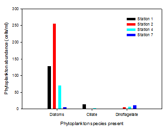
Figure 6 -
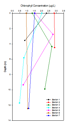
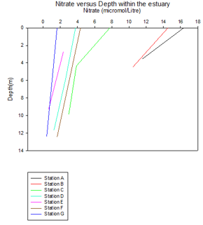
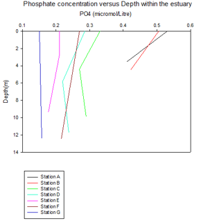
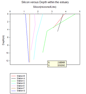
Figure 7 -
Figure 7 -
Figure 8 -
Figure 9 -
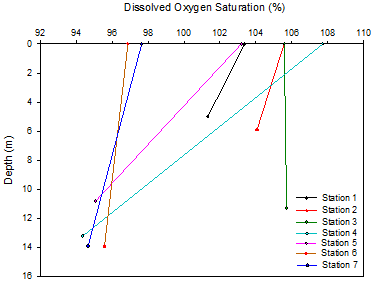
Figure 10 -
Estuarine Mixing Diagrams
The Fal estuary has two river inputs, the River Fal and Truro River which have different
discharges. The freshwater endmembers are rough estimates of the two rivers mixing
without being influenced by seawater. Surface salinities from station 1 at Black
Rock were used for the marine end-
Theoretical dilution lines were plotted on each mixing diagram to identify whether
conservative or non-
The nitrate mixing diagram does not represent the entire estuary, but for the areas
sampled, there appears to be non-
The phosphate mixing diagram shows a slightly non-
The silicon mixing diagram displays non-
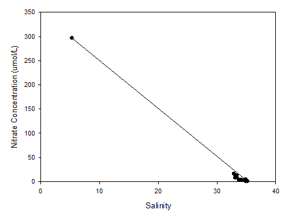
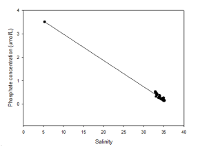

Figure 11 -
Figure 12 -
Figure 13 -
- Perillo, G. (1995). Geomorphology and sedimentology of estuaries. Amsterdam: Elsevier.
- Stoermer, E. and Smol, J. (1999). The diatoms. Cambridge, UK: Cambridge University Press.
- Wang, Y., Zhang, W., Lin, Y., Cao, W., Zheng, L. and Yang, J. (2014). Phosphorus,
Nitrogen and Chlorophyll-
a Are Significant Factors Controlling Ciliate Communities in Summer in the Northern Beibu Gulf, South China Sea. PLoS ONE, 9(7), p.e101121. - Kiørboe, T. (2011). What makes pelagic copepods so successful?. Journal of Plankton
Research, 33(5), 677-
685. - Nixon, S. W. and Pilson, M. E.Q. 1983. Nitrogen in Estuarine and Coastal Marine Ecosystems. Nitrogen in the Marine Environment. Section III: Systems. Chapter 16.
- Thamkatrakoln, K. and Hildebrand, M. 2008. Silicon Uptake in Diatoms Revisited: A
Model for Saturable and Nonsaturable Uptake Kinetics and the Role of Silicon Transporters.
Plant Physiology. 146(3):1397-
1407. - UK Marine Special Areas of Conservation. Phosphorous. [Online].
Available from: http://www.ukmarinesac.org.uk/activities/water-quality/wq9_2.htm
[Accessed on: 28th June 2015] - NOAA. (2014). What is an Estuary. [Online].
Available from: http://oceanservice.noaa.gov/facts/estuary.html
[Accessed on: 1st March 2015] - Officer C. B. and Ryther J. H.(1980). The Possible Importance of Silicon in Marine
Eutrophication. Marine Ecology-
Progess Series. Vol: 3. Pages:83-91 - EPA. (2006) Voluntary Estuary Monitoring Manual, Available from:
http://water.epa.gov/type/oceb/nep/upload/2009_03_13_estuaries_monitor_chap10.pdf
[Accessed on: 28th June 2015]
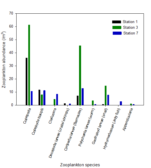
Figure 5 -