
Falmouth 2015 Group 10
The aim of this survey was to investigate the physical, chemical and biological, structure of the Fal estuary from the upstream station, 29 (as far upstream as vessel and conditions would allow) to Black Rock - station 35 - a marine end member station.
A CTD was deployed at each station to collect samples for later analysis, with phytoplankton samples extracted at 5 of the 7 stations and a zooplankton net deployed at 3 stations (stations 29, 32 and 35), chosen to have a suitable representation of the changing species richness and abundances along the river and estuary.
The samples were collected and analysed later in the lab - to view the methods of collection and sampling for both the estuary and offshore, please click HERE.
This information could then be used to examine the behaviour of the estuary as a transition between the freshwater River Truro and its tributaries, and the English Channel, by determining the level of mixing within the estuary, and the variations in flow throughout.
Through analysis of the changing plankton community organisation throughout the Fal, the impacts of factors such as salinity, temperature and nutrient concentrations on the estuarine biota can be determined.
Date: 26-06-2015
Time: 07:00 UTC
Location: Fal Estuary (various)
High Water: 12:15 UTC
Low Water: 18:10 UTC
Tidal Range: 3m
Sea State: Calm (0)
Average Wind: 7 Knots
Prevailing Wind: South westerly
Cloud Coverage: 7/8th
Vessel: RV Bill Conway

The biological aim of the investigation was to gain a general overview of the biomass, biodiversity and community structure of the plankton in the Fal estuary. A CTD was deployed at each station to take in-situ measurements, and Niskin bottles were attached to the rosette to collect samples for later analysis of chlorophyll, oxygen and nutrients. Sample depths were chosen during the lowering of the CTD to find potential points of interest in the water column.
Limitations
Contamination- chlorophyll filters were stored in acetone immediately after being used, but may still have been affected by spray or rainwater,
and innaccurate volume measurements may affect analysis- most water
measurements were taken using volumetric flasks (as opposed to pipetting). Weather, sea swell and human error could all contribute to different volumes of water being passed through the filter.
Possible Improvements
Identifying phytoplankton could be achieved by a less time-consuming method such as that put forward by (1), where it would have been possible to sample more phytoplankton groups, possibly gaining a more complete picture of the estuary, or of multiple depths at a single station. However, the pigmentation method does not identify the phytoplankton to a species or genus level, making biodiversity analysis less meaningful.
A time series of each station over the course of a tidal cycle could account for some unexplained variation , especially regarding the balance between riverine and oceanic inputs.
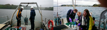
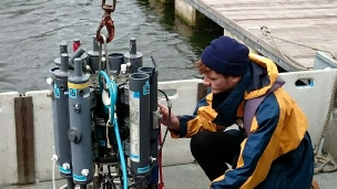
The CTD apparatus (with Niskin bottles) being deployed by crane from the back of RV Bill Conway.
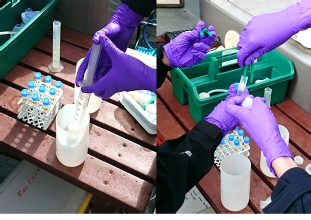
Filtering of estuarine water by hand, and the storage of the filters in 90% acetone.
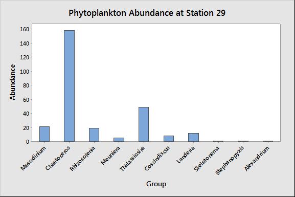
Station 29 - top of the estuary (total: 276)
This station is also dominated by diatoms, most of which are the colonial Chaetoceros. This is possibly due to the spring bloom. Dinoflagellates however, have a relatively low diversity in the estuary, potentially being out competed by the diatoms, which are able to assimilate nutrients at a faster rate (depending on the light conditions). Station 29 was the furthest up the river, which (in theory) should have the highest nutrient concentrations. This would explain the large diatom numbers, as they are less prone to be limited by nutrients if they are closer to the source. In this station, the low diversity and abundance of dinoflagellates might be due to out competition for nutrients by diatoms. The dominant species, Chaetoceros occupied 57.45% of the phytoplankton population.
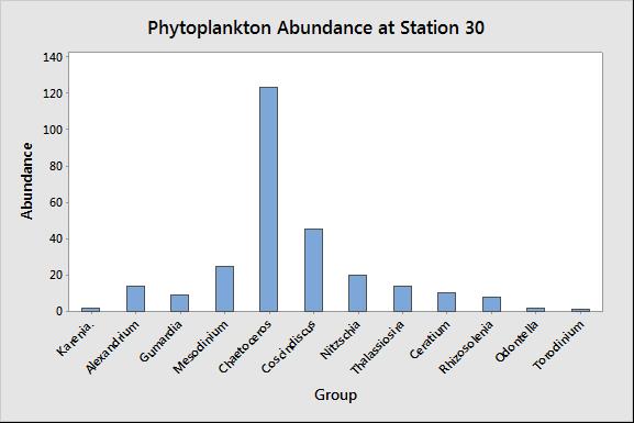
Station 30 – where the Truro river meets Fal river (total: 275)
This station is dominated by diatoms, most of which are colonial Chaetoceros. Their dominance may be representative of the spring phytoplankton bloom. However there is also a strong dinoflagellate presence and diversity. This could mean that silicate is limiting diatom growth while other groups like dinoflagellates proliferate as the other nutrients are still available. The site corresponds to where the Truro River and the Fal river meet up, which would be an area of concentrated nutrients. This may explain the phytoplankton abundance and diversity. Chaetoceros occupied 45% of the phytoplankton population.
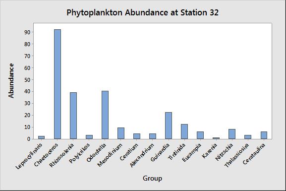
Station 32 - mid estuary (total: 241)
Station 32 has the highest diversity of all stations observed. Yet again, the phytoplankton is dominated by diatoms (spring bloom). The high diversity may be the result of the concentration of phytoplankton by riverine and tidal action focusing a variety of different species into one area. The “low” numbers could be explained by a decrease in nutrient concentration as they are consumed further upriver. Diatoms are still the major constituent of the phytoplankton, but are not as dominant as the previous stations. This may be due to a decrease in silicon concentrations closer to the mouth of the river. Chaetoceros had the highest abundancce again at 41%.
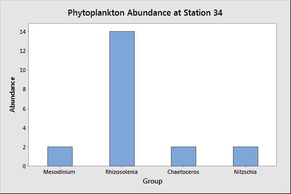
Station 34 - main estuarine basin
Station 34 was particularly poor in phytoplankton abundance and diversity. However the high numbers of phytoplankton observed at stations either side of this one suggest that they may have been grazed. Chaetoceros only occupied 10%, with Rhizosolenia being the most abundant.
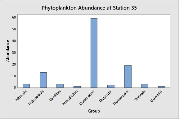
Station 35 mouth of the estuary – black rock (total: 104)
Station 35 was at the mouth of the estuary; therefore lower phytoplankton numbers and diversity are expected. This station was the furthest surveyed from the main nutrient source (the river) and it exhibited the lowest abundances and diversity of all sites surveyed. Yet again, the phytoplankton are dominated by diatoms (spring bloom), while a variety of dinoflagellates are also present in low numbers. Unlike previously, the low abundance of dinoflagellates might be due to nutrient depletion by consumption further up the river rather than out competition from an available pool of nutrients. Chaetoceros 57.84%.
To view a table of phytoplankton abundances for each station, please click here.
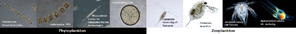
Phytoplankton (click on each image to enlarge or view as slideshow)
Zooplankton (click on each image to enlarge or view as slideshow)
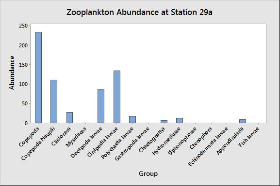
Station A (most riverine)
Copepods, small crustaceans that are found in fresh and seawater habitats are the dominant group at Station 29a, making up 36.7% of the species collected. These are important to the global carbon cycle as they feed on phytoplankton and contribute to the carbon sink at the ocean surface. The cladocera, commonly known as water fleas, and cirripedia larvae were also numerous, consisting of 17.3% and 21.1% respectively.
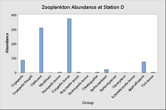
Station D
Cirripedia larvae, the meroplanktonic juvenile form of barnacles, were the dominant species, with 42.5% of the species collected. The cladocera were also plentiful, comprising 35.4% of the sample, which is surprising as most are fresh water species, with only 8 species being truly oceanic. This may be because they are outcompeted by the copepods in the fresher water area of station 29a and are pushed toward the middle of the estuary, where the copepods do not seem to thrive as much, making up only 10% of the sample, most likely due to other species outcompeting them.
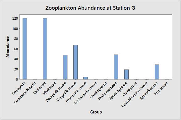
Station G (full seawater salinity)
Copepods and the cladocera were equally abundant at Station G with 26.3% each of the sample. Cirripedia larvae comprised 14.7%, but there were more marine groups than at the previous stations, including hydromedusae (10.5%), decapod larvae (10.5%) and siphonophorae (4.2%). This is expected as the water here is fully saline.
To view a table of zooplankton abundances for each station, please click here.
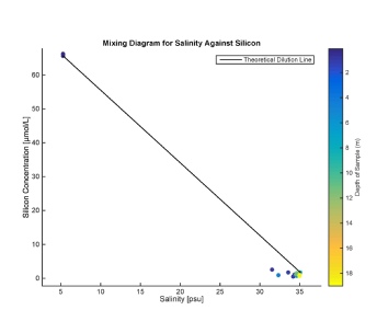
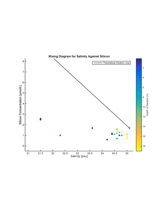
Silicon
The results show that dissolved silica levels generally decrease as salinity increases, which is due to weathering of silicate rocks that increase riverine concentrations in comparison to seawater. The Fal is well-mixed tidally dominated estuary and therefore the salinity differences are slight, making it harder to interpret. For this reason the 'zoomed in' graph gives a better picture of the dissolved silicon levels. At the most landward sample site [station 29], dissolved silica concentration is approx. 2.5 µmol/L but at station 35 it is only slightly lower at approx. 1µmol/L. Comparison with the Theoretical Dilution Line shows that dissolved silicon behaves non-conservatively and is removed from the estuary. This is probably due to uptake by siliceous phytoplankton, such as the abundant Chaetoceros diatom. The results also show that similar concentrations of dissolved silicon were collected throughout the water column. This could be attributed to the powerful mixing processes in the Fal estuary that make the water column more homogenous.
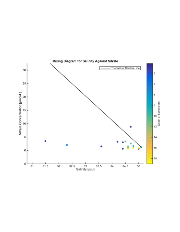
Nitrate
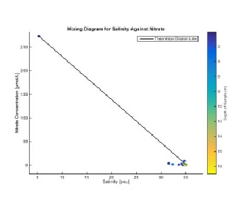
The results show that nitrate concentrations in the Fal estuary also show con-conservative behaviour. Using the ‘full’ graph we can see that the stations sampled are all strongly tide dominated with typical values of nitrate concentration far lower than the riverine end member. Looking at the ‘zoomed in’ graph we can see that nitrate concentrations all plot at around 0-5 µmol/L, far below the Theoretical Dilution Line which probably indicates biological removal by primary producers. The final stations at the estuary mouth also show that, apart from one anomalous point, nitrate was uniformly mixed from the surface to 18m depth.
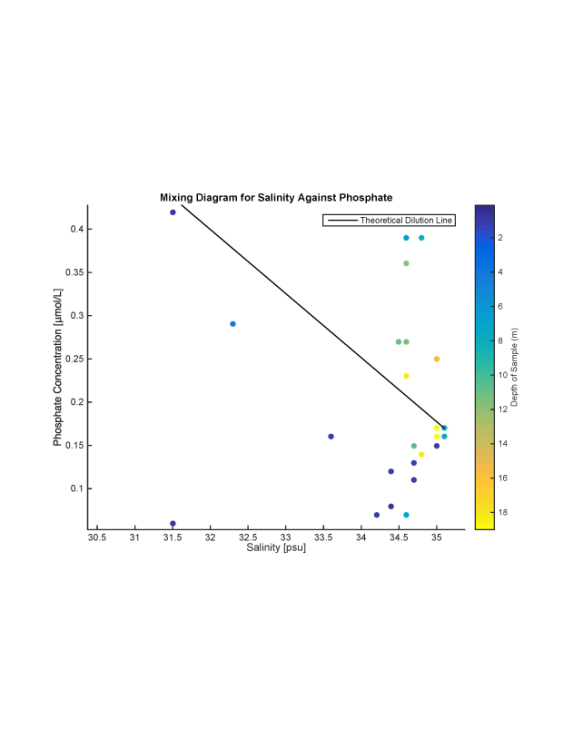
Phosphate
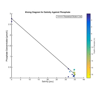
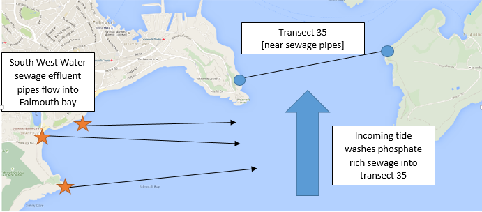
The results show that Phosphate concentrations in the Fal estuary do not have a conservative behaviour pattern. Typical concentrations ranged from around 0.4 µmol/L at station 29 down to around 0.1µmol/L at station 35 at the estuary mouth. At the early inshore stations in the estuary, phosphate concentrations plot below the Theoretical Dilution Line indicating removal over this flushing timescale. This is likely caused by high levels of biological primary productivity depleting the nutrients in the water column. At the mouth of the estuary near Black Rock there is an anomaly. Using the ‘zoomed in’ graph from 0-6m depth there are still depleted levels of phosphate, but from 6-18m there seems to be addition of phosphate up to 0.25-0.35µmol/L. Contrasting with this result, there is no similar spike in nitrate for the same stations. A source of phosphate that would not increase nitrate concentrations could be urban sewage waste from pipes to the west of the estuary mouth. Modern sewage systems tend to properly remove nitrate from sewage but is not as efficient at removing phosphate. After consulting ‘The Environment Agency’ and contacting ‘South West Water’ group 10 were given 3 sets of co-ordinates for sewage pipes that flowed directly into Falmouth Bay. The addition of sewage close to the transect and the fact that the tide was in flood explains how the additional phosphate was washed into sample station 35 to artificially raise the background phosphate above expected levels.
Figure showing the effluent sources for urban sewage in the Fal Bay
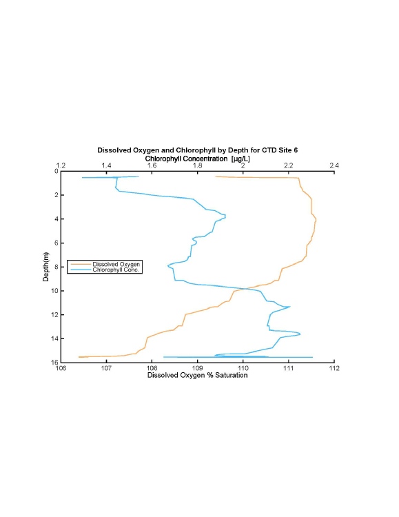
Chlorophyll and Oxygen
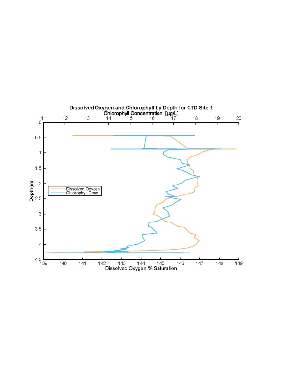
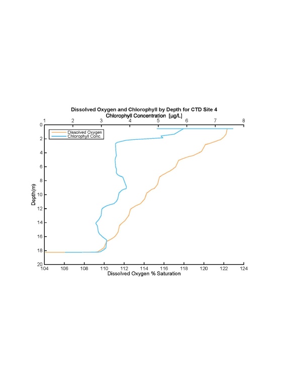
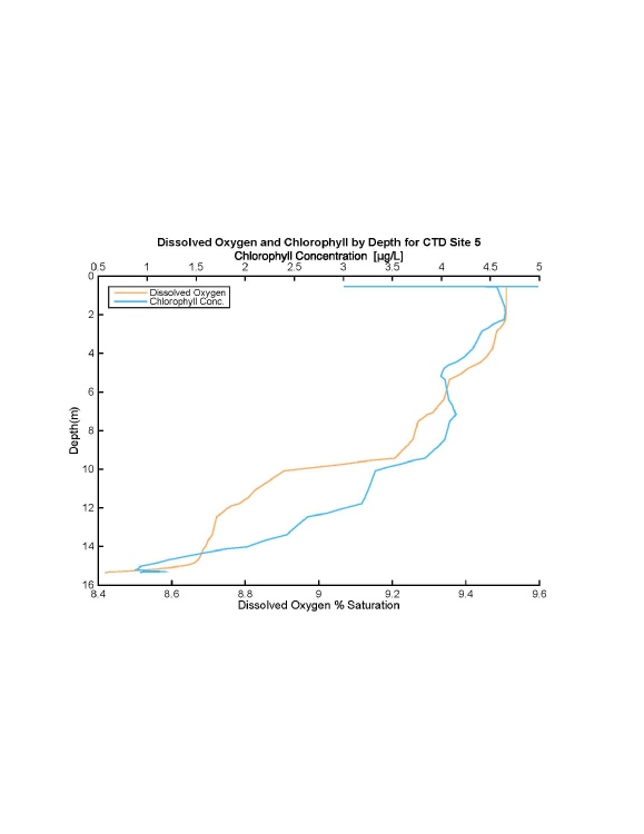
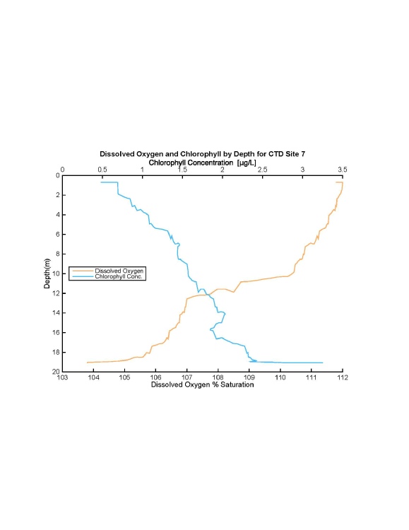
Chlorophyll concentration decreases at all depths from the river end to the marine end of the estuary. Near-surface concentrations were measured at around 15.8µg/L at Site 1, decreasing to 5.8µg/L at Site 4. At the mouth of the Fal, Site 7, chlorophyll concentration had dropped to 0.5µg/L.
At most of the sites surveyed, chlorophyll decreases with depth. However, at both Site 1 and 5, there is a subsurface chlorophyll maximum, before the concentration begins decreasing. At site 1, this occurs at 2m, where around 18µg/L was recorded. At Site 5, this is less pronounced, with a peak at 2m less than 0.1µg/L greater than that of the surface sample.
At Sites 6 and 7, the typical profile is reversed, with chlorophyll tending to increase with depth. At Site 6, this increase is from 1.45µg/L at the surface, to a peak of around 2.25µg/L at 14m. At Site 7, the 0.5µg/L surface measurement increases to 2.25µg/L at 19m.
At every site, dissolved oxygen saturation decreases with depth, as at the surface, oxygen is replenished by the atmosphere whereas in unmixed deeper water only photosynthesis prevents respiring organisms from removing the entirety of the dissolved oxygen. The most rapid change occurs at Site 2, where saturation decreases from 140% at the surface to 110% at 11.5m. Overall oxygen saturation decreases with distance down the estuary, with a maximum of 147% at Site 1, compared to a maximum at Site 7 of 112%. However, at Site 5, a short term, rapid loss of oxygen is observed, with a maximum of 9.5%. Fairly low chlorophyll was also measured here, meaning that eutrophication is not likely to be the cause.
Click photos to enlarge
Graphs and discussions of initial findings from ADCP, CTD and Secchi disk data collected while on the RV Bill Conway.
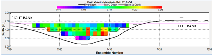
ADCP
Data was collected from stations 29 through 33 on a flood tide, and stations 34 and 35 on an ebb tide, which is reflected in both the flow velocities and directions on the ADCP data. For all of the ADCP transects, please click HERE.
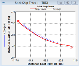
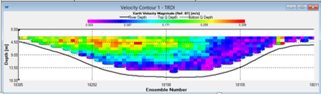
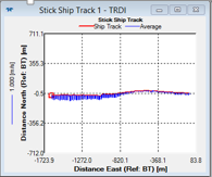
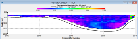
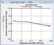
Station 29 (Top) 5 Averaged
The direction of flow is uniform down the river, as measurements were taken during the flood tide, though the speed of flow is variable with both depth and distance along the transect, as shown by the range of velocities shown in the data. The fastest flow was seen at an intermediate depth along the left bank, whereas the areas of slowest flow were at the surface and bottom of the water column; the latter possibly owing to friction with the riverbed.
Station 30 (at fork in river to two confluences) 5 Averaged
This transect took place very close to a fork in the river where two confluences were present, accounting for the high total discharge of 480.55m³. The slowest flow was found along the right bank, with the fastest in the surface waters to the left of the channel, and a gradient of velocities in between. This may be due to the friction from the right bank and the narrow channel of the right confluence slowing the flow, with faster flow at the left on the surface due to the left confluence having a wider channel, and so less friction entering the confluence.
Station 31 (two creeks to left) 5 Averaged
Station 31 showed a similar flow pattern to the previous station, possibly due to the influence of two creeks at the left of the channel. A ‘pocket’ of faster flow travelling upstream can be seen between the surface and about 12m depth to the left of the river, with the fastest flow occurring at 4m below the surface. This may be due to the influence of the creeks, causing the sea water to tend towards the creeks (as the tide was coming in). The right bank shows a different scenario. There is an area of slower flow ‘hugging’ the right bank and extending across the river bed to the left bank, which is flowing in the opposite direction to the fast flow, suggesting that this is riverine flow towards the estuary. The slower flow is partly due to being on flood tide, and partially due to friction.
Station 32 (At Channals Creek)5 Averaged
There are two obvious areas of very slow flow, with the fastest flow occurring towards the bed of the estuary in the middle of the transect. Directionality of the flow suggests that water is mainly travelling towards the East, almost across the estuary, potentially caused by the seawater that has entered the creek, exiting again and travelling in a different direction than if the creek was not present.
Station 33 (widening of river into estuary)10 Averaged
Total transport for this station was larger than the previous due to the sudden widening of the channel. The flow measured along this transect is almost homogenous, with only small variations in the main channel. The flow speed was much slower at this location as the tide was approaching high tide slack water, and so flow up river was decreasing before the direction reversed. Net transport for this station is North-East, with little variation throughout the transect and water column.
Station 34 (tide turned, mid-estuary)15 Averaged
At the time of data collection, the tide turned and so total transport was extremely low (at 23.03m3) in the downstream direction. Flow speeds and directions along the transect vary little, with flow speeds not exceeding 0.1m/s, due to seaward flow power beginning to exceed upstream flow though the two dips in the channel show slightly higher flow, which may be explained by less friction being caused by the seabed and banks.
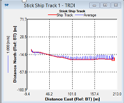
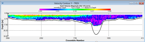
Station 35 (Black rock)15 Averaged – Should be flipped 180 degrees.
The total transport at Black Rock exceeded 1500m3 seaward as it is located at the mouth of the estuary where the channel is very wide, allowing for large volumes of water transport. Flow velocities seem to be fairly uniform at the left of the channel at all depths, and in the lower few meters towards the right of the channel, with highest flow velocities occurring in the upper 6m at the right of the deepened channel. As with the previous station, the flow is unidirectional in the seaward direction, as high water had passed and the tide was now in the ebb phase.
CTD
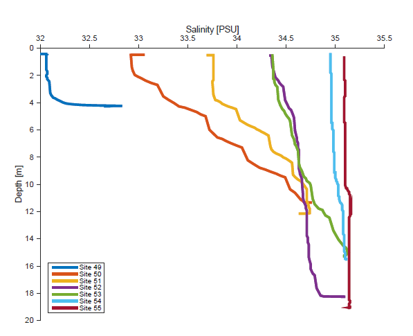
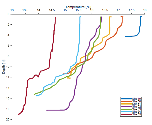
As the stations move further from the riverine and into the marine section of the estuary, the salinity of the water increased and the temperature decreased. This would be because of the increasing influence of the marine system. This also caused an increase in the mixing of the water column, as indicated by the earlier station numbers have a larger halocline than those closer to the sea. The minimum salinity recorded at any station was 32, implying that at the time the measurements were taken the marine inputs were the most influential. This was because the tide was coming in during the time the stations furthest from the marine system were taken. Click the images to enlarge.
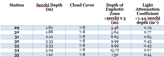
Secchi Disk
The secchi disk data from the estuary shows that light attenuation decreases from the riverine to the marine end of the estuary. The depth of the euphotic zone increases moving toward the marine end of the estuary. This is likely due to the higher nutrient concentrations from riverine input available for biological uptake which in turn means higher levels of phytoplankton and therefore more light attenuation. The data collected from stations 32 and 33 is exactly the same. This could be due to the change in sea state at this time; with slight roughness, heavy rain and sea state of 2 at station 32; to fairly choppy and a sea state of 4 at station 33. The cloud cover was very thick all day, likely reducing the depth of the euphotic zone, and the weather worsened from calm and dry in the morning (sea state of 1); to heavy rain and swell waves (sea state of 4) towards the end of the day.
RICHARDSON NUMBERS
The Richardson number is a dimensionless number defined as the ratio between the density gradient and velocity shear. When Ri > 1, the flow can be considered stable and laminar. If Ri < 0.25 it is described as turbulent.
The following graphs show the relationship between Richardson’s numbers and depth at stations 30, 33 and 35. These stations were chosen as they are the two end members and the middle station, to cover all estuarine conditions.
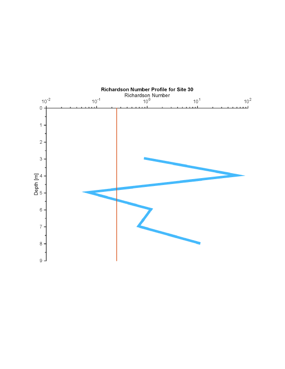
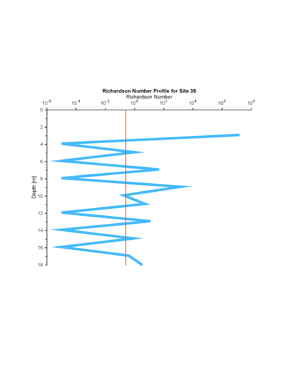
All figures have a red line indicating the point where Ri = 0.25, the boundary between laminar flow (<0.25) and the beginning of turbulence. Turbulent flow is only certain if Ri > 1. Click on the figures to enlarge with captions.
Flow is turbulent from the shallowest point of the measured area, reaching a maximum Richardson number of nearly 100 at 3.9m, indicating extremely turbulent flow. The flow then rapidly alters into a laminar layer, before finally becoming turbulent again at the greatest depths measured.
The top and bottom layers of turbulence are likely due to wind-driven forces at the surface and friction with the estuary bed at depth. This effect can be seen across the estuary except at the middle site (site 33), possibly due to calmer conditions during sampling.
Station 30 is the most riverine of the stations sampled for Richardson number, and represents the most turbulent flow. The station is located near a secondary riverine input (running in a different direction the main flow), which would increase turbulence. In addition to this, the more riverine nature of the station means that the riverine flow is significant enough to interfere with tidal flows, which are almost entirely dominant at lower points in the estuary. As the tide was coming in while the measurements were taken at this station, the interactions between these two bodies of water would have increased the turbulence.
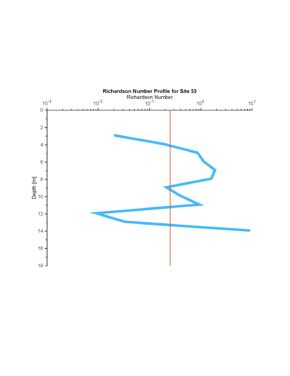
Station 33 shows laminar tendencies near the surface, becoming partially turbulent between 4-11m. This becomes laminar with depth until the deepest point is reached, where massive an amount of turbulence occurs.
The layers of station 35 rapidly change from laminar to turbulent with every metre of depth travelled down, with the most turbulence occurring near the surface. This is indicative of the large number of influences (especially tidal) all converging upon a relatively shallow area.
1.1- Schluter, L.; Mohlenberg, F.; Havskum, H.; Larsen, S. (2000). The use of phytoplankton pigments for identifying and quantifying phytoplankton groups in coastal areas: testing the influence of light and nutrients on pigment/chlorophyll a ratios. Marine Ecology Progress Series, 192, 49-63
2- Nagadomi, H., Kitamura, T., Watanabe, M., & Sasaki, K. (2000). Simultaneous removal of chemical oxygen demand (COD), phosphate, nitrate and H2S in the synthetic sewage wastewater using porous ceramic immobilized photosynthetic bacteria. Biotechnology Letters, 22(17), 1369-1374.
3- Environment Agency, 2015. Industrial Pollution- Interactive Maps. [Online]
Available
at: http://maps.environment-agency.gov.uk/wiyby/wiybyController?x=180500.0&y=32500.0&topic=pollution&ep=query&scale=7&location=Falmo uth,
Cornwall&lang=_e&layerGroups=1&distance=1&textonly=off
[Accessed 2 July 2015].
4- South West Water, 2008. SWW Draft Water Resources Plan 2008. [Online]
Available
at: http://www.southwestwater.co.uk/media/pdf/a/f/Section_1.pdf

The views on this website are solely those of Group 10, and are in no way affiliated with the views of University of Southampton or the National Oceanography Centre.
 BACK TO TOP
| Introduction |
| Metadata |
| Biological |
| Chemical |
| Physical |
| References |
| Introduction |
| Metadata |
| Biological |
| Chemical |
| Physical |
| References |
| Introduction |
| Metadata |
| YSI |
| Flowmeter |
| Chlorophyll a |
| Irradiance |
| References |
| Introduction |
| Metadata |
| Methods |
| Sidescan |
| Video Ground-Truthing |
| Poster |
| References |