Introduction:

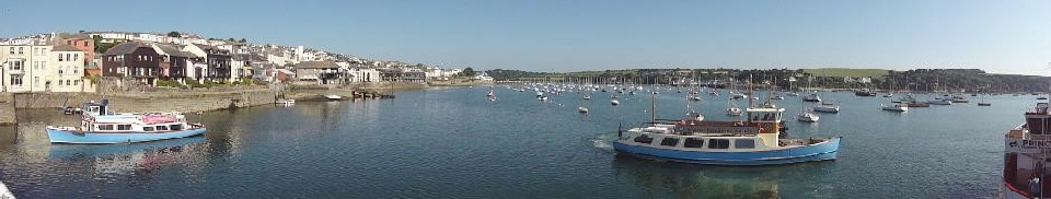
Offshore from Falmouth, the sea is relatively exposed and subject to south-westerly winds from the Atlantic. Here, mixing is high and so the input from the Fal estuary is quickly diluted. However closer to Falmouth, the sea is more sheltered due to the geography of the area. In order to investigate how conditions change going away from the shore, frontal systems around Falmouth were investigated. This investigation was carried out by Group 1 on the 23/06/2014, who investigated various physical, biological and chemical parameters. The instruments used were a rosette CTD, an ADCP, and a plankton net. Biological data from the rosette sampler, and the plankton samples were analysed the next day in the labs.

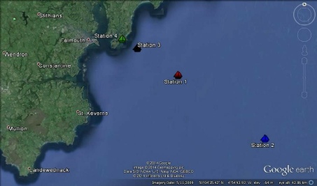
The aim of the survey was to investigate the features of tidal fronts. Four stations were observed, locations of which are shown in Figure 2. The stations were more stratified offshore, and became more mixed the closer they were to shore. The physical, chemical, and biological structure of each of these stations varied, and are discussed in detail below.

Positions of stations (Figure 1):

Station 1 - Latitude: 50o 05.71’N

Longitude: 004o 52.17’W

Time: 10.43 UTC

Station 2 - Latitude: 50o 00.30’N

               Longitude: 004o 40.75’W

               Time: 13.20 UTC

Station 3 - Latitude: 50o 08.00’N

               Longitude: 004o 57.52’W

               Time: 15.48 UTC

Station 4 - Latitude: 50o 08.77’N

               Longitude: 004o 59.51’W

               Time: 16.38 UTC

Physical

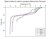
Temperature - Figure 2

The temperature profiles all show a decrease in temperature with depth.

Station 1 has a steep thermocline at 15-20m depth. It has a large top to bottom temperature difference with the surface temperature of around 18oC and a bottom temperature of around 12.5oC.

Station 2 temperature profile has a similar structure to that of Station 1; it has a steep thermocline at 18-22m and a large top-to-bottom temperature difference of surface temperature at 18.3oC and bottom temperature at of 12.0oC.

Station 3 has a multi-layer thermocline with distinct layers between 0-5m, 7-18m, 20-25m, and 30-38m. This station is in between being well-mixed and strongly stratified. i.e. the mixing processes are large enough to mix parts of the water column, but not mix the whole column to a homogeneous temperature.

Station 4 is the most inshore profile. It is continuously stratified, with a steady decrease in temperature from 0-10m from 18.1oC to 16.8oC. It is at an intermediate stage between well-mixed and stratified.

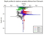
Salinity - Figure 3

‘Salinity spiking’ can be seen in Figure 3. This is caused by a mis-match in the measurement of conductivity and temperature, rather than a real feature of the water column. Ignoring the spiking, the general trend of salinity can be observed. Stations 3 and 4 are slightly fresher than Stations 1 and 2 as they are further inshore (see map).

Station 1 has lower salinity in the surface (31.15) and constant salinity of 35.20 from ~5m to the bottom at 65m. The range of the change (0.05) is relatively very small, but may have been caused by freshwater input via rainfall.

Station 2 has relatively constant salinity with depth, and again has slightly lower salinity in the surface which could be due to freshwater input.

Station 3 has higher salinity in the surface (0-10m) which decreases between 10 and 30m by ~0.1. The salinity increases between 30 and 40m by 0.1. The change of salinity is relatively small, and would not affect the stability of the water column in comparison to the change in temperature (~4oC).

Station 4 has constant salinity of 35.15 throughout the water column. The water column is well-mixed at this station.

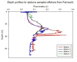
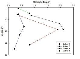
Fluorometry - Figure 4

The fluorometry depth profile shown in Figure 4 indicates where the chlorophyll maxima are in the water column. As a trend, the amount of fluorescence is lowest (0.05 v) from the surface to 20m depth.  The fluorescence peaks at a depth around 30 to 40 m. This peak is shown in Station 1, 2, and 3. Station 1 has the highest peak in fluorescence and Stations 2 and 3 have similar values. Station 4 has a different profile: this station was taken in much shallower waters next to the coast line (measurements reach a depth of only 10 m) resulting in lower fluorescence values of 0.1v compared to 0.32v maxima at Station 1.

The chlorophyll appears to accumulate at a depth where the temperature is lower and below the thermocline. As shown in Figure 2, the thermocline occurs at a depth between 18–20 m. Fluorometry peaks occur just below this depth, this allows the phytoplankton to utilise the nutrient-rich waters below the thermocline.

Figure 2: Offshore temperature profile

Figure 4: Offshore fluorometry profile

Station 1 (11:10-11:14 UTC)

As shown in Figure 5, the velocity changes significantly within the water column. There is a surface layer of water down to 15m with variable velocity, a band of water with higher velocity 0.2m/s at around 15-20m depth, and below this the water column has velocities of <0.1m/s. This station was the second furthest station from the mouth of the estuary.

At Station 1, backscatter has a highest value of around 80 [dB], this layer extends from 5m to 18m depth (Figure 6).

Station 2 (13:30-13:36 UTC)

Station 2 was station furthest from the mouth of the estuary. This station shows higher velocities throughout the water column compared to the others. Between 0–20m the velocity is highest (0.4m/s), and below 20m it drops to a lower range of 0.175 – 0.350 m/s (Figure 7).

The highest amount of backscatter is seen just below the surface at 5 m, as shown in Figure 8. This trend is clearly shown at Stations 1, 2 and 3, however at Station 2 the backscatter in the deeper water column is higher than 1 and 3.

Station 3 (15:55-15:56 UTC)

Station 3 was closer to the mouth of the estuary than Station 1 and 2. There is a sub-surface layer of lower velocity water (0.06m/s) at 10-15m depth, and water of higher velocity below this layer (Figure 9). This was different to the other stations measured: velocities went as low as 0.05 m/s. The water column here has a sub-surface layer of lower velocity water (0.06m/s) at 10-15m depth, and water of higher velocity below this layer.

Backscatter (Figure 10) shows a similar trend to the first 2 stations.

Station 4 (16:42-16:43 UTC)

Station 4 was just outside of the estuary mouth. This also shows a lower and more constant velocity profile, shown in Figure 11. The velocity is mostly 0.075-0.175 m/s.

The layer of higher backscatter at this station extends from the surface to 5m depth (Figure 12), compared to the other stations where the layer was sub-surface.

Velocity

At Stations 1 and 2, the layer of higher velocity located between the surface and 20m is consistent with the depth of the thermocline and changing temperature with depth. The increased velocity is due to shear between the wind-driven layer and the deeper water.  Station 4 was much shallower, and the water more mixed; there was little change of temperature and salinity with depth and the velocity also has little variation.

Station 3 - Unlike the first two stations that were surveyed, the distinct layer at Station 3 was of lower velocity than the surface and deeper water. One hypothesis that could explain this is related to internal waves. The breaking of an internal wave, unlike a surface wave which has a backwash component on a beach due to gravity, does not occur along a gradient - meaning that it simply has forward momentum until the energy disperses. In the water column, if this momentum is in the same direction as the water current, then the velocity will increase relative to the surrounding water. Conversely, if the momentum of the breaking wave is in an opposing direction to the water current the velocity will be lower. This could be what is happening at Station 3 with the layer of lower velocity.

Backscatter

Backscatter indicates where there is a high amount of matter in the water column that reflects back. This matter can indicate detritus, zooplankton and suspended sediment. After looking at the zooplankton, it can be seen that the zooplankton vertical tow from 25-0m at Station 1 has a lower abundance than the 40-30m tow. This suggests that the backscatter shown may also be due suspended particulate matter. At Station 2 and 3, the distribution of zooplankton in the water column is more consistent with the location of higher backscatter in the upper metres. For example at Station 3 there is a higher zooplankton abundance in the 10-0m tow than the 35-10m tow. The Station 4 vertical tow covered the whole water column from 10-0m, so we cannot say that the backscatter in the surface 5m is just due to zooplankton; it is likely to have also been suspended particulate matter due to the close proximity to the coast and the shallow water depth.

Chemical

Phytoplankton are at the base of the ocean food web, and require nutrients, light and carbon dioxide in order to photosynthesize and grow. The main nutrients (macronutrients) are nitrate, phosphate, and silicate. Coastal waters are generally eutrophic (nutrient-rich) as nutrients are introduced to the water via rivers.

During winter months, decreased solar irradiance and increased winds cause the water column to fully mix. Phytoplankton are light-limited during these months, as they are unable to stay in the euphotic zone, where there is enough light to facilitate growth. Solar irradiance increases during spring and winds are weaker, which leads to warming at the surface of the water column. This leads to stratification as a warmer surface layer sits above the cooler, denser bottom layer. The phytoplankton bloom during this time utilize the nutrients in the surface layer, and nutrients below the euphotic zone remain high. Commonly, after the spring bloom, there is a peak in chlorophyll at the thermocline. This is where light conditions are just enough for growth, and nutrients are introduced via diapycnal mixing.

Station 1 is stratified with a thermocline at ~12-22m. At 38m, there is a fluorometry maximum shown by the CTD data (Figure 4). This peak in fluorometry matches with the high chlorophyll and silicate concentrations (Figure 19). The nitrate concentrations are relatively lower at this chlorophyll peak; however it is not fully depleted. The peak of chlorophyll indicated by the fluorometry profile and the chlorophyll concentrations, corresponds to the depth of the euphotic zone which was measured to be >36m using a secchi disk. At depth, the phytoplankton become light-limited leading to the observed low chlorophyll and higher silicate, phosphate, and nitrate concentrations. Oxygen would be expected to be higher at the chlorophyll peak; however the results show an oxygen minimum at the chlorophyll maximum (Figure 20). This could be due to high respiration at this depth.

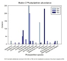
Station 2 is stratified with a thermocline between 15 and 23m. There is a chlorophyll maximum below the thermocline at 32m, which is similar to the calculated euphotic zone depth (31.2m). This is coupled with an O2 maximum, which is expected due to the production of O2 during photosynthesis (Figure 20). There is high nitrate (Figure 17), phosphate (Figure 18), and silicate (Figure 19) concentrations at the depth of the chlorophyll maximum, which are likely to be facilitating the bloom. The high chlorophyll concentrations at this depth may be due to an increase in light penetrations through the water column, which could be facilitated by higher solar irradiance, calmer weather, or a decrease in suspended particles.

Station 3 is thermally stratified with a step structure of temperature; it is at a mixing stage in between mixed and stratified, with multiple mixed layers and small temperature gradients. The euphotic zone extends through the whole column (calculated using the CTD as a secchi disk). There is high chlorophyll at 24m and at 32m (Figure 21). Oxygen is high in the surface, which may be due to waves causing mixing, and low at the bottom, which may be due to remineralisation (Figure 20). Phosphate (Figure 18) and silicate (Figure 19) increase with depth, and nitrate is highest at 24m (Figure 17). Nitrate is depleted at the bottom of the water column, which corresponds with the chlorophyll peak. The chlorophyll may therefore be due to old growth, as further phytoplankton growth would be limited by the nitrate.

Station 4 is the most inshore profile, it is 10m deep and is continuously stratified. As at Station 3, the euphotic zone extends through the whole water column. Chlorophyll is highest at the bottom of the water column (10m), which is matched by an increase in O2 (Figure 20). Nitrate (Figure 17) and silicate (Figure 19) are highest in the surface of the water column, which may be due to input via rivers. Phosphate is higher at 10m than at the surface, however (Figure 18). The high chlorophyll at depth, but low nitrate, may show that the chlorophyll maximum at 10m is due to older growth.

The chlorophyll peaks at Stations 1 – 3 are below the thermocline (Figure 4 and 21), which is different to the expected pattern of a peak within the thermocline. This may be due to increased light penetration due to less mixing, or increased solar irradiance. The euphotic zone depths, which were calculated using the secchi disk method, are deep in to the water column.  

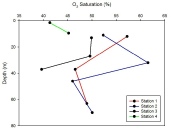
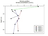
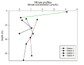
Figure 17: Offshore nitrate profiles

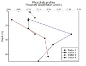
Figure 18: Offshore phosphate profiles

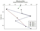
Figure 19: Offshore silicate profiles

Figure 20: Offshore oxygen profiles

Biology

As seen in Figure 21, the chlorophyll levels increase with depth, peaking to a chlorophyll maximum at depths of around 30 m which decreases again as you move down the water column, this is shown at Stations 1, 2 and 3. Station 3 has higher the highest Chlorophyll concentrations, and Station 2 is considerably lower.  Station 1 shows as sharp increase from 0.4 µgrams/L near the surface to a maximum of 1.9 µgrams/L at 37 m. As chlorophyll concentration acts as an indicator for phytoplankton concentration the pattern shown helps to support the phytoplankton counts below that suggest higher numbers of phytoplankton at depth which are similar (around 30 -35 m), and explains why the amount of chlorophyll generally decreases with depth as there are fewer phytoplankton capable of living there (due to insufficient light and nutrients).

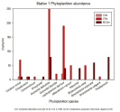
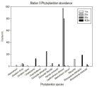
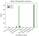
Phytoplankton

The overall trend of phytoplankton compositions off shore show low phytoplankton abundance in the surface and shallow waters. For Stations 1, 2, and 3 the amount of phytoplankton increases to its highest at a depth of around 30 – 37 m deep. These stations were in open ocean waters with clearer stratified waters. Here, elevated numbers of phytoplankton are seen just below the thermocline and are also indicated by the high levels of Fluorescence and Oxygen concentrations and lower Nitrate concentrations also at similar depths. Phytoplankton communities are dictated by chemical, physical and biological properties, these include nutrient availability, light levels, predators and grazing, temperature and water column mixing levels.

Leptocylindrus danicus and Guinardia delicatula occur the most through the offshore survey. Station 4 was much shallower, resulting in more constant phytoplankton numbers through the water column. This is because there is not an opportunity for the water column to become stratified like it would in deeper offshore waters where stronger thermoclines and nutriclines can develop. Looking at the Chlorophyll graph (Figure 21), we can see that Station 4 does in fact increase at depth but there is no peak in Chlorophyll, probably because Station 4 was only 10 m deep. There are noticeably higher concentrations of Leptocylindus dancius and Rhizosolenia spp that are just below and equal to 1000 cells/ml for depths of 1.4m and 9.5m (Figure 28). Station 4 is better mixed (shown by Temperature and Salinity profiles), resulting in a high number of the diatom Rhizosolenia spp which are more suited to this kind of environment.

Hydromedusae and Copepoda appear to thrive when Leptocylindrus dancius and Guinardia delicatula are the dominant phytoplankton.

Conclusions from these samples are limited as it only represents a fraction of the entire plankton community. Human error could possibly occurred through personal interpretation during the identification process.

Richardson number

The Richardson number (Ri) is a dimensionless parameter used to estimate the water column stability, and represents the relative importance of static stability and dynamic instability. It compares the relative magnitude between stabilizing forces of the density gradient and the inertial flow forces, and can be calculated using Equation 1.

W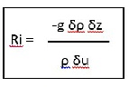here g is gravity (m/s²), H is the water column depth (m), ρ0 is the average density (kg/m³), δρ is the density change with depth and δu is the horizontal velocity gradient  with depth (m/s) (Knauss, J. 1997).

Ri > 1 is the limit from which the flow is described as laminar, where buoyancy forces tend to overcome the inertial forces and stratification of the water column can be found, whereas Ri < 0.25 describes turbulent flows, i.e. the energy provided by the shear flow can be used to overcome the density gradient and vertical mixing as well as shear between the interfaces promoting entrainment can occur in the water column. An intermediate state is found between 0.25 < Ri < 1, where both stratification or mixing is likely to occur.

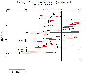
In Figures 13-16, the Richardson number values were calculated for each meter depth and are shown in logarithmic scale. The density data was given by the CTD measurements at each station, while the horizontal velocity was given by the ADCP. For the calculations where the velocity gradients were tending to zero, the values were out of scale and in order to improve the interpretation, they were excluded from the graphs. Also, in order to use the logarithmic scale, negative Ri values were changed to zero.

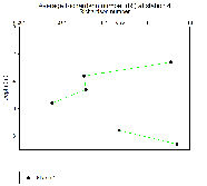
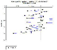
At stations 1, 2, and 3 (Figures 13, 14, and 15) the higher Richardson numbers (Ri > 1) were correlated with the position of the thermocline, representing the stratification caused by the temperature gradient and the influence of the buoyancy input near the surface. Station 2 was located at the tidal front, therefore showing some stability in the top 10 meters depth as a function of the salinity distribution in addition with the solar energy input. 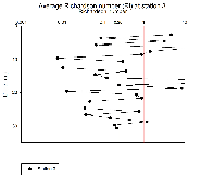Also, below the thermocline the lower Ri values (Ri < 0.25) were correlated with the almost constant temperature distribution indicative of vertical mixing. Overall, most of the Ri values for station 3 were below the 0.25 limit, showing that turbulent mixing caused by winds and tides overcome the stratification, except at the thermocline between around 12 and 25 m depth. Station 4 was much shallower (10.7 m) and consequently more well-mixed.

Figure 3: Offshore salinity profile

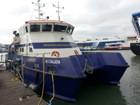
Offshore data was collected on the vessel RV Callista (pictured above)

Figure 1: Location of Stations  1-4

Figure 13: Average Ri number at Station 1

Figure 14: Average Ri number at Station 2

Figure 15: Average Ri number at Station 3

Figure 16: Average Ri number at Station 4

Equation 1

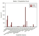
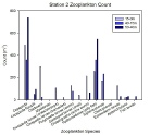
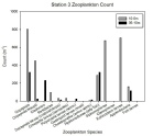
Zooplankton

Zooplankton also bloom at certain depths for each station. However the blooms are notably not at the same depth range as the phytoplankton blooms. Station 1 and 2 (Figure 23 and 25) were the furthest stations offshore and also the deepest. At Station 1, the highest numbers of zooplankton were found between 40 – 30 m, and for Station 2 zooplankton are most abundant between 50 – 40 m.

At both of these stations, Hydromedusae and Copepoda were the most commonly identified species: at Station 2 there was 750 m^-3 Copepoda and 575 m^-3 Hydromedusae.  Zooplankton will peak if there is a large food source (a peak in phytoplankton). They will do this just below the apparent phytoplankton peak so to utilise it. Station 3 (Figure 27) was closer to the main land and was different to the first 2 stations as zooplankton levels peaked between 10 – 0 m and are mostly made up of Echinoderm larvae (800 m^-3), Siphonophores (700 m^-3) and Copepoda.

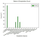
Fewer numbers of zooplankton species were found at Station 4 (Figure 29) but at higher concentrations; Copepoda  (130 m^-3), Decapoda, Cinepadia larvae  and Polychaeta larvae.  Zooplankton show seasonal variations. Copepods are the most common zooplankton found throughout the offshore survey, this is not surprising as they are the most abundant metazoan occurring in the ocean (Davies et al. 1999). The differences here are due to the differences in water column mixing and current that will affect what phytoplankton and zooplankton are adapted to living there.

Similar compositions of phytoplankton produce similar compositions of zooplankton as different phytoplankton will encourage different predators. Examples of this can be seen in Stations 1 and 2 (Figure 22 and 23, and Figure 24 and 25).

Figure 21: Chlorophyll depth profiles for each station

Figure 22: Station 1 phytoplankton

Figure 23: Station 1 zooplankton

Figure 24: Station 2 phytoplankton

Figure 25: Station 2 zooplankton

Figure 26: Station 3 phytoplankton

Figure 27: Station 3 zooplankton

Figure 28: Station 4 phytoplankton

Figure 29: Station 4 zooplankton

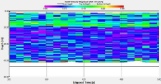
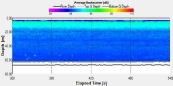
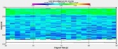
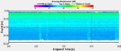
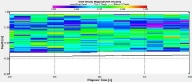
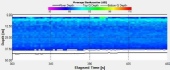
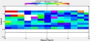
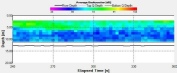
Figure 5: Station 1 Velocity

Figure 7: Station 2 Velocity

Figure 8: Station 2 Backscatter

Figure 9: Station 3 Velocity

Figure 10: Station 3 Backscatter

Figure 11: Station 4 Velocity

Figure 12: Station 4 Backscatter

Figure 5: Station 1 Backscatter

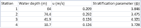
Stratification index

The stratification parameter (ɸ) is another estimation of the degree of stratification of the system as a result of the balance between the tidal currents, which tend to stir the water column, and the energy provided by the buoyancy input in order to maintain any degree of stratification. It represents the work required per unit volume to completely mix the water column. It can be calculated using the equation:

ɸ = log10(H/u³), where H is the average water column and u is the measure of the strength of the tidal currents by using the tidal stream range from the tidal diamond chart near Plymouth.

Values of the stratification parameter higher than 2 (ɸ > 2) indicate strong stratification, whereas complete vertical mixing will be expected if ɸ < 1. The transitions between the two regimes, i.e. the tidal mixing fronts, seem to occur in all cases close to a value of ɸ ≈ 1.5 (Pingree and Griffths, 1978).

As seen on the temperature profiles from the CTD data, all stations showed stratification along the thermocline, with some steep gradients on station 2 and 1, from about 10 to 25 m depth. The higher values for ɸ, different from what should be expected for tidal front regions like Station 2 for instance, are maybe due to the uncertainty and estimation of the tidal currents from the tidal charts. For example, the distance between this station position (50°00’.3 N, 004°40’.8 W) and the tidal stream F position (50°02´.5 N, 004°58´.8 W) used to calculate its tidal current, as well as the difference in the water column depth (Station 2 was 10 meters deeper than the expected water column of tidal stream F) could explain the higher ɸ value for station 2 (ɸ = 3.475), when compared to the values more commonly found on tidal mixing fronts (ɸ ≈ 1.) (Pingree and Griffths, 1978) or to the critical  = 2.7 suggested by Simpson and James (1986).

Reference: Simpson, J.H. and James, I.D. (1986). Coastal and estuarine fronts. Baroclinic Processes on Continental Shelves, 63-93.

Pingree, R.D. and Griffiths, D.K. (1978). Tidal fronts on shelf seas around the British Isles. J. Geophys. Res. 83 (C9), 4615-4622.

Simpson, J.  and Sharples, J. (2012). Introduction to the Physical and Biological Oceanography of Shelf Seas, , Cambridge University Press, Cambridge, UK

Knauss, J. (1997). Introduction to Physical Oceanography. 2nd edition Prentice-Hall Inc. New Jersey.