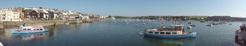
The Fal estuary is the 3rd largest natural harbour in the world. Formed from the drowning of a river valley at the end of the last ice age, it has freshwater inputs from the Rivers Carnon, Kennal, Penryn and Truro. These fluxes of freshwater inputs, together with the strength of the tidal current and the wind driven mixing in the water column contribute to the extent of stratification in the estuary.
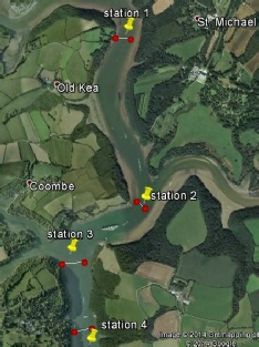
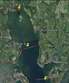
In order to determine the physical, chemical, and biological structure of the estuary and its nutrient environment, Group 1 conducted a survey at 7 different stations (Figure 32 and 33) on 28th June 2014, starting from Malpas Point down to Black Rock at the mouth of Carrick Roads.
Vessel: RV Bill Conway
High Tide 06:02 UTC (4.55m) Low Tide 12:47 UTC (1.01m)
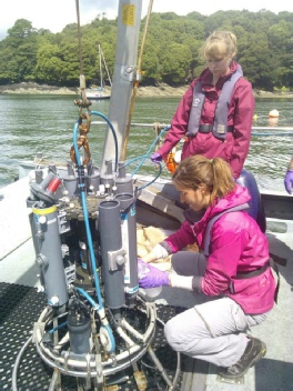
On arrival at each station a CTD was used to give a vertical profile of the water column, Niskin sample bottles were collected at various depths and processed for chemical analysis of phosphate, silicate, nitrate, dissolved oxygen and chlorophyll. We studied the water column from the CTD profile and chose sample depths accordingly. Additionally, an ADCP transect was taken at each site to provide information on velocity across the estuary, and a secchi disk depth was estimated. At Stations 1, 4, and 7 a 200um mesh net was used to collect plankton (inner diameter 50cm), this was due to analysis time constraints.
Temperature -
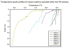
Surface temperatures in the upper estuary are higher than the lower region by approximately 0.7 Celsius degree. Temperatures are relatively constant in the water column in stations 1, 2, 3 and 4. Stations 5, 6 and 7 show a structure, possibly representing a stratification pattern.
Temperatures measured in the first four stations are slightly higher than those found on the three last stations. These stations also have a constant temperature in the water column, which indicates that either water is well mixed or that the whole water column is being heated. In this case, it is probably due to mixing, because by analysing salinity graphs, it is possible to notice that salinity profiles have patterns of well mixed estuaries and as this region is shallower than the other, mixing occur in the whole water column.
The lower estuary, which is closer to the open ocean is also deeper and more affected by tidal currents. Temperatures lowers with depth, but the highest difference found between surface and bottom was at Black rock station (Station 7) and it was of 2 Celsius degrees, which indicates that the estuary has a pattern of weak stratification.
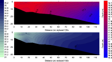
The top graph on Figure 35 represents the transect corresponding to all stations along the estuary and presents the spatial variation of temperature both along the depth and the length of the estuarine channel. It is possible to observe in this figure that temperature decreases seaward and at increased depths. Also, it is important to notice that the horizontal distance stated in the figure is reduced by 100 (one hundred) times, for reasons of scale.
Salininty -
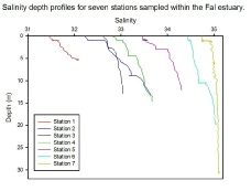
In Figure 6, it is possible to observe that there is a variety of salinities ranging from 32.0 at the upper part of the estuary (Station 1) to 35.2 at the mouth of the estuary (Station 7). From Station 1 to Station 7 the surface salinities increase in order as the stations approach the open ocean. At all stations, the surface water can be seen to be lower at the surface than in the deeper water.
As expected, the salinities increase in order from Station 1 to Station 7 as the stations approach the open ocean. However, the range of salinities from the upper to the lower part of the estuary is small. This is due to the fact that the riverine input to the Fal Estuary has been very small in the weeks preceding the study, which means that the process of dilution of seawater as it enters the estuarine environment is slowed down.
It can be seen in the graph that the salinity increases with depth in all stations. This is because fresher water is less dense than more saline water and so the fresher water is at the surface whereas the more saline water is found in deeper water. The salinity profile structure also depends on the type of mixing in the estuary. In the first five stations, the salinity varies quite a lot with depth. This means that these stations are quite well stratified. Stations 6 and 7 have less variety in salinity with depth, and so are more mixed. This is because the closer to the open ocean the stations are, the greater the influence of tidal mixing.
The bottom graph in Figure 35 also corroborates these findings and allows the visualisation of a slightly pronounced salt wedge into the estuary.
TS diagrams -
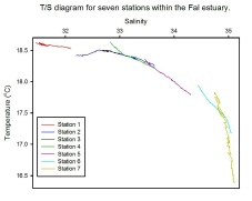
Generally, all TS profiles are straight lines, which indicates that there is only one type of water mass in the profile. First four stations are constant in temperature, while salinity changes with depth and stations close to the open sea have their salinity constant, while temperature changes with depth.
TS profiles clearly show that the estuary is well mixed, because all profiles are almost straight lines, indicating there is no stratification in the upper estuary. In the lower part of the estuary, there is a small sign of stratification, since these stations are closer to the open sea and more affected by tidal currents. One factor that is important to be considered is that these last stations were done in low tide, so probably in high tide, the scenery would be different.
Fluorometry -
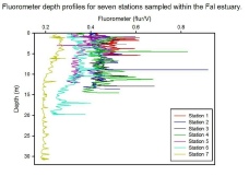
In the Fal estuary, the fluorometer readings vary greatly both between and within stations. In general, there is an increase in the fluorometer readings from Station 7 (which was done closer to the ocean) to Station 1 (which was done at the head of the estuary). Although the graph may be quite difficult to interpret due to the many spikes in data at many of the stations around 0.4flur/V, a general trend is observed with peaks at middle depths and at the bottom for almost all stations with exception of Station 7 and Station 5. Station 7 does not show any significant peak and Station 5 has its highest peak near the surface, and then decreases as it gets deeper.
Richardson Number -
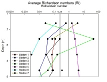
The Richardson numbers (Ri) correlate well with the temperature profiles for all stations, indicating a laminar flow in most of them as a result of weak stratification. Stations 1, 2, 3 and 4 all showed Ri values in the turbulent region (Ri < 0.25). This pattern is expected as the depth is lower at the top of the estuary, varying between 7.3 m at station 1 to 16 m at station 2, promoting a strong vertical mixing. In addition, these stations showed maximum vertical gradients of about 0.4 °C for temperature and 1.3 PSU for salinity, which explains the weak vertical density gradients found, hence giving low Ri values. At station 5, on the other hand, the flow was laminar (Ri > 1), which was due both to the spread of the flow following the geology of estuary and also because this station was done at approximate low tide, where the flow changed direction and got weaker. Further outwards of the estuary, the flow was laminar (Ri < 0.25) at station 6 and stratified at the top first meters for station 7, with turbulence taking place further deep. This can be explained by the fact that stations 6 and 7 were done after low water, with increasing tidal current velocities that enhance turbulent mixing.
Depth Profiles
Nitrate -
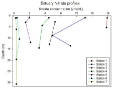
As you can see, going from Station 1 (at the fresher-
At Station 1, the concentration is the highest since this station is the furthest upstream. The nitrate concentration is highest upstream since the main sources of nitrate are land based. At stations further downstream, the concentrations gradually decrease as the nitrate is utilised by algae and phytoplankton for growth. At station 7 (near the open ocean) the concentration of nitrate is fairly uniform with depth, which shows that the water column here is quite well mixed. In stations 1, 2, 3, 4 and 5 the nitrate concentration decreases from the surface measurement to the measurement at the next depth. This is because the phytoplankton do not live right at the surface, but a bit deeper. This peak in phytoplankton deeper in the water column can be seen as a chlorophyll maxima on other graphs. Therefore, the nitrate concentration is higher at the surface since less of it is being used up since phytoplankton can not live here due to the high level of irradiance.
Phosphate -
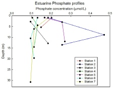
In this graph, you can see that the phosphate concentrations are very variable between stations. There seems to be no clear pattern. Phosphate is an element found in high concentrations in rocks and soil. Therefore it would be expected that the concentration would be the highest at Station 1, and the lowest at Station 7 as the stations sampled move further away from the terrigenous source of phosphate. However this pattern is not seen in this graph. It may be due to the concentration being so low (eg all seven stations having concentrations in the range between 0.0µmol/L and 0.5µmol/L) that it is hard to see any pattern.
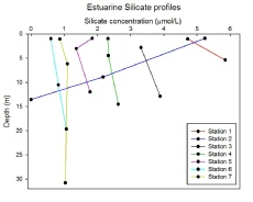
Silicate -
Silicate is used as you move down the estuary from the river end to the open ocean end. Looking at the profile, Silicate is highest at the stations near the river end: Station 1 has a Silicate concentration of 4.8 µmol/L which reduces to 0.6 µmol/L by Station 6 and 7 which were by the estuary mouth head. This is because Silicate is taken up by phytoplankton, in particular Diatoms that need it to make exoskeletons. Looking at the estuary phytoplankton graphs the major phytoplankton are found across the sampled stations are diatoms, particularly Chaetoceros (the most abundant phytoplankton), Thalassiosira and to a lesser extent Guinardia delicatula. It is these diatoms that remove the silicate in the water.
As you move down the water column at each station the silicate concentration remains relatively constant (apart from minor fluctuations, Station 1 indicates an increase as you move down the water column, suggesting it is being added faster than it is removed).
The major exception from the trends identified is Station 2. It has a surface Silicate concentration that is high (5.2 µmol/L) which is what is expected as it is nearer the river end. However this concentration does not stay the same as you go down the water column but in fact reduces to almost 0 µmol/L. This suggest something is removing the Silicate down the water column and not replenishing it. This is unusual and could be attributed to human error.
Oxygen -
The percentage of oxygen at each station is higher at the surface. This is due to
oxygen production from primary production and diffusion of oxygen from the atmosphere
across the sea-
The oxygen saturation seems to be decreasing drastically at Station 5, this might be due to the high rate of respiration. However, no sampling was taken for zooplankton at this station; hence this hypothesis cannot be confirmed. The decrease in oxygen concentration might also be due to decomposition of organic matter by bacterial respiration. A various number of sewage water are discharged in the upper estuary; this impacts the microbial water quality and provides substrate for microbial respiration.
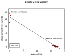
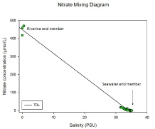
Mixing Diagrams -
Estuarine mixing and subsequent exchange with adjacent coastal waters are fundamental physical processes governing biological, chemical, and sediment interactions within coastal and estuarine systems. During estuarine mixing phases, if a linear relationship exists between the concentration of a particular dissolved constituent and a conservative indicator of mixing between sea water and fresh water (e.g. salinity), then the behaviour of the constituent can be described as conservative. Conversely, any deviation from the conservative behaviour will be indicative of either addition or removal processes (Burton, et al. 1970).
The mixing diagrams for silicate (Figure 45), phosphate (Figure 46) and nitrate (Figure
47) can be used to determine whether the Fal estuary is behaving conservatively (dominated
by physical processes) or non-
Looking at the three figures to the right Silicate and nitrate concentrations were much higher for the riverine end members and decreased as the salinity increased in the area sampled. Silicate and nitrate seem to behave conservatively, with values following the theoretical dilution line. Phosphate also had some higher values for the riverine end members when compared to the sampled values, but unlike silicate and nitrate, it does not seem to behave conservatively, which might be due to the fact that there is a sewage treatment station, which discharges sludge with high nutrient content, near the Truro River, a tributary to the Fal estuary.
References: Burton, J., Liss, P. and Venugopalan, V. (1970) The behaviour of dissolved
silicon during estuarine mixing I. Investigations in Southampton water. Journal du
Conseil, 33(2), pp.134-
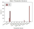
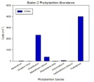
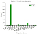
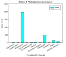
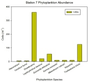
Phytoplankton -
Overall, the same species of phytoplankton, Chaetoceros and Thallasiosira, can be seen in higher abundances at all stations throughout the estuary. Both these most common phytoplankton are shown to general decrease in abundance from the head to the mouth of the estuary.
Chaetoceros shows a general decrease in abundance from the head to the mouth of the estuary, with the exception of Station 2. This could be because the sample was taken at a much deeper position in the water column and a decrease in phytoplankton is expected due to low nutrient concentration.
Thallasiosira abundance is very high in Stations 1 and 2, at the head of the estuary. However, in all other stations the abundance is much lower. Analysis of the data can suggests that Thallasiosira thrives in high nutrient conditions.
Many other species were found at all stations, however their abundance is too low to be able to draw conclusions about their distribution along the estuary.
The conclusions drawn from the data collected in the estuary may have limitations as human error may have occurred during the phytoplankton identification process. Furthermore, the data counted was only a very small subsample of the estuary. One rare species may have been identified and then extrapolated to show a higher abundance than actually exists.
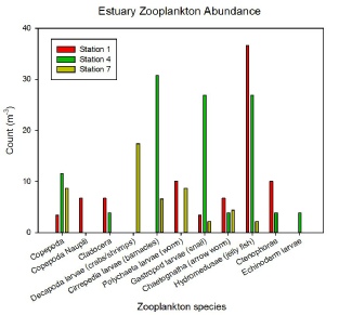
Zooplankton -
Zooplankton distribution and abundance changes along the estuary, with some species observed only at certain areas of the estuary while others were observed throughout the estuary at varying abundances. For example, the abundance of Chaetognatha stayed relatively similar at all stations samples, which may suggest a cosmopolitan distribution along the estuary.
On the other hand, Copepoda nauplii were only identified in the zooplankton sample taken at Station 1 in the head of the estuary, whereas Copepoda were more abundant further down the estuary in Station 4 and Station 7. This observation can suggest that the head of the estuary acts as a nursery ground for this species until individuals are big enough to move down the estuary.
Hydromedusae were also found at a higher abundance in one area of the estuary. They occurred more often at the head than at the mouth of the estuary, which could suggest that this species requires a higher input of nutrients in order to thrive.
A high abundance of decapoda larvae was found strictly at Station 7, which is the mouth of the estuary. This could be because of salinity limiting the range of decapoda larvae to the higher salinity found at Station 7.
Although the data may imply plausible conclusions, human error during the identification process and identifying only a very small subsample of the estuary may limit the reliability. Due to the small subsample used to identify zooplankton, echinoderm larvae were only found in the middle of the estuary at Station 4. Perhaps this larvae would have been identified if a larger part of the sample taken at Station 1 and Station 7 was observed.
Flushing Time and Discharge -
Both flushing time and residence time give an approximate indication of how long a parcel of water or particle reside in the estuary before being forced out of the estuary. However, the residence time is more affected by the river discharging rates while the flushing time significantly correlates to the tidal flow. Since, the survey was carried out as the tide was receding (HW; 06.02 and LW; 12.47), the flushing time for each station was calculated. Important assumption when calculating flushing time: none of water removed from the estuary during the ebb tide returns to the estuary during the next flood tide.
Flushing time = [(V)estuary/(V)prism] x (T)tidal
(V)prism x (A)estuary = h
Where h is the tidal range (HW – LW), h in this case is 3.9m
= 6.45h (23,220s)
The area in between stations was approximately calculated using google earth while the average depth at each station was taken from the CTD data. The vessel did a transect near each station and the discharge of water out of each station was estimated by the ADCP.
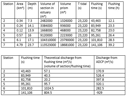
Considering the table above, the flushing time is larger at Station 6 and 7. At these stations the water is deeper, causing the water to get mixed over a longer span of time before being flushed out. Similarly a shallower section of the estuary (Station 2) experiences a lower flushing time while sections of the estuary with the same depths undergo the same flushing time (Station 3 and 4).
The theoretical discharge was also calculated using the flushing time. The theoretical discharge does not correlate with the discharge from the ADCP data. This is because the theoretical discharge averages the discharge from HW to LW on the tidal cycle while the ADCP data represents the instantaneous discharge at a specific point on the tidal cycle. The theoretical discharge corresponds to the instantaneous discharge at maximum velocity flow (midpoint between HW and LW). The biggest difference between the two discharges occurs at slack point (either at HW or LW). This is clearly shown by Station 6 and 7, both surveyed at low tide (tidal chart).
There is a large difference between the theoretical discharge and the measured one at these two stations. Moreover, the negative discharge measured by the ADCP imply that water is flowing in the opposite direction. This is because the water is starting to flood into the estuary after low tide.
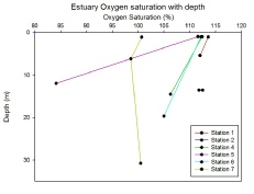
Figure 32: Map of stations 1, 2, 3 and 4.
Figure 33: Map of stations 5, 6 and 7.
Students operating CTD rosette and Niskin bottles
In situ fluorometry is frequently used in oceanography to provide depth-
The stations closer to the open ocean have lower fluorometry values than in the estuary. This is because there is higher nutrient concentrations in the estuary which equates to higher chlorophyll/fluorometry values.
Figure 34: Temperature profiles
Figure 35: Temperature and salinity transects
Figure 36: Salinity profiles
Figure 37: TS diagrams
Figure 38: Fluorometry
Figure 39: Average Richardson numbers (Ri)
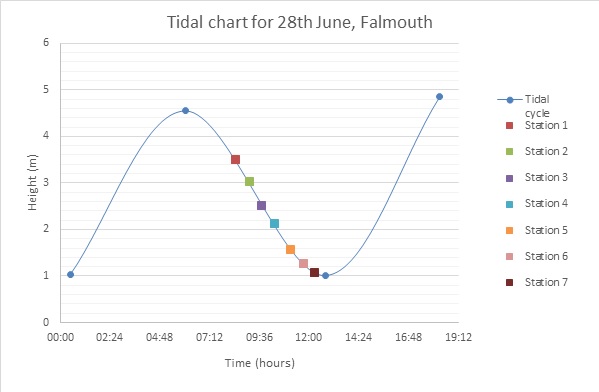
Figure 40: Tidal chart for the day of estuarine sampling
Figure 41: Nitrate profiles
Figure 42: Phosphate profiles
Figure 43: Silicate profiles
Figure 44: Oxygen profiles
Figure 45: Silicate mixing diagrams
Figure 45: Nitrate mixing diagrams
Figure 46: Phosphate mixing diagrams
Figure 52: Estuarine zooplankton
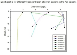
Figure 46: Chlorophyll depth profile
Figure 47: Station 1 Phytoplankton
Figure 48: Station 2 Phytoplankton
Figure 49: Station 4 Phytoplankton
Figure 50: Station 6 Phytoplankton
Figure 51: Station 7 Phytoplankton