


Figure 1: Time series of irradiance (mmol photons m-2s-1)
against depth (m) at 50˚12’58’’N, 005˚1’40’’W
Station 1: 11.05UTC, Station 2: 11:46UTC, Station 3: 13:04 UTC.
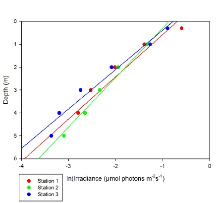
Figure 2: Natural log of irradiance (mmol photons m-2s-1) against depth (m) with linear regression line for each station, taken at 50˚12’58’’N, 005˚1’40’’W Station 1: 11.05UTC, Station 2: 11:46UTC, Station 3: 13:04 UTC.

Irradiance
The irradiance depth profiles (Figure 1) display how light attenuates exponentially with depth at each station. From plotting the natural log of the ratio of depth to surface sensor reading against depth, a linear decrease of light with depth can be observed and the slope of the linear regression line used (Figure 2) to estimate the attenuation coefficient (kd) at each station. These estimates (0.54, 0.46, 0.58 for station 1 2 and 3 respectively) reveal how light attenuation fluctuates slightly but remains relatively constant over the time series. The 1% light depth was calculated for each station (8.5m, 9.96m and 7.93m for stations 1, 2 and 3 respectively) again showing little change.
The physio-chemical conditions in an estuary are highly variable and it is within the mid-estuary that this variability is highest. These changes in physio-chemical conditions, affects the survival and distribution of estuarine fauna. This physiological stress can be inferred from changes in biota’s distribution within the estuary over time, as organisms move to stay within their preferred physiological zone.
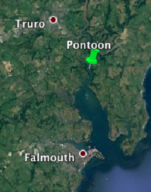
Collecting data for a range of physical, chemical and biological variables over time from a fixed point within the estuary allows the relationship between these variables to be tested. In this investigation, a pontoon (50 12’58’’N 005 1’40’W) in the mid-estuary of the Fal estuarine system will be used to create a time series over the tidal cycle. This investigation aims to create water column profiles measuring physical characteristics such as water flow, light attenuation, turbidity and oxygen saturation, and biological characteristics such as chlorophyll concentration in order to establish how the physical, chemical and biological components of the estuary change over time. The relationship between these components will then be investigated.
Cloud cover was 8/8 Intermittent light rain HW 12:57 LW 19:10


Turbidity
Turbidity (Figure 3) shows a fairly uniform depth profile throughout the time series, with highest turbidity in the top 1m of the water column (0.8NTU) which then generally decrease to 0.6 throughout the rest of the water column. From 11:09 UTC to 1149 UTC a marked increase in turbidity occurs between 3 to 4m, peaking at 1.2NTU at 11:30 UTC.
This is most likely caused by a ferry or other vessel leaving the pontoon creating a wake which stirs up the sediment temporarily increasing turbidity (Hilton and Phillips, 1982). The increase in turbidity could explain the increase in light attenuation at station 2 (11:46 UTC) due to increasing scattering of light.
Chlorophyll
Chlorophyll was measured from filtered samples of the water column at 1 hour intervals
at the same location using a Niskin Bottle. The sample was filtered through a filterhead
on a 50ml pipette and the filter was then submerged in 6ml of 90% acetone sample.
The samples were transferred to a freezer and stored for 12 hours.
Results
Chlorophyll was most concentrated between 1-2m with a peak concentration at
*m at 11:** UTC as seen in Figure (contour plot chlorophyll pontoon).
The flooding tide before the high tide at 12:57 UTC mixed the water column and influenced the decrease in chlorophyll concentration, starting at lower depths and then mixing closer to the surface. The warmer, fresh river water flows over the colder, salty dense water that penetrates the lower depths, increasing with the flooding tide (Figure 4). After the high tide the water column mixed again and chlorophyll concentration increased at a lower depth due to the ebbing tide.
Oxygen
Oxygen was measured using a YSI multiprobe in the same location at 1 hour intervals.
Results
Oxygen concentration is highest at the surface (Figure 5) and remains fairly
stable throughout the timescale, this could indicate activity of photosynthetic organisms
during daylight hours. The highest percentage oxygen saturation recorded was 113%
at a depth of approximately 1.5m. There is an overalll decrease with depth due to
photosynthesis at the surface producing oxygen as a by-product and respiration occuring
at depth, using up oxygen. Tidal input caused the percentage oxygen saturation to
increase at the surface, the contour plot shows that at high tide, dissolved oxygen
increases.
Temperature
The results show that there is a buoyant surface layer of warm water, and temperature decreases with depth (see Figure 6). Riverine water tends to be warmer than seawater, cold water is dense so sinks through the water column. The water column is stable but stratified as layers are distinguishable in the contour plot, the strong thermocline aids the suspension of phytoplankton in the euphotic zone. The temperature change is attributable to the effect of solar radiation and land radiation which relates to the heat budget components latent heat from evaporation and sensible heat loss.
Salinity
Figure 7 shows that the Fal Estuary is a salt wedge, where salinity is higher at the mouth and lower at the head. There is a large difference between salinity at the surface and at depth, the highest salinity reading is 34 and the lowest is 32.5. The figure indicates that there is a well-developed halocline where the riverine input is greater than the seawater input. Throughout the time series the tide was flooding, but it is evident from the contour plot that the tide turned, as salinity at the surface starts to increase at approximately 11:49 UTC, revealing a stronger inflow from the saline sea water. This could be explained by a time lag in tides as tide times were calculated from Falmouth and the King Harry Pontoon is not in the same location, therefore the tide may have been ebbing, causing an increase in salinity at the surface.

Figure 6: Contour time series of Temperature (°C) against depth at location 50˚12’58’’N, 005˚1’40’’W Sample 1: 11.00 UTC, Sample 2: 11:37 UTC, Sample 3: 11:57 UTC
Figure 5: Contour time series of Percentage Oxygen Saturation against depth at 50˚12’58’’N, 005˚1’40’’W Sample 1: 11.12 UTC, Sample 2: 12:09 UTC
Figure 4: Contour time series of Chlorophyll (ug/L) against depth at 50˚12’58’’N, 005˚1’40’’W Station 1: 11.00 UTC, Station 2: 11:37 UTC, Station 3: 11:57 UTC.
Figure 3: Contour time series of turbidity (NTU) against depth (m) at location 50˚12’58’’N, 005˚1’40’’W Sample 1: 11.00 UTC, Sample 2: 11:37 UTC, Sample 3: 11:57 UTC.

Figure 7: Contour time series of Salinity against depth at location 50˚12’58’’N, 005˚1’40’’W Sample 1: 11.00 UTC, Sample 2: 11:37 UTC, Sample 3: 11:57 UTC
At 11:27, flow was fairly slow at the surface and stronger in deep water. Flow was to north in the surface waters and to the north in deep water (Figure 8(a)). At approximately 3m depth, flow velocity is extremely low at around 0.022ms-1 . The direction flow also reverses at this depth. At 12:04 the flow was much stronger at the surface.
Flow was in a north direction throughout the water column (Figure 8(b)). At 12:45, flow was slower at the surface and at 5m depth. The direction of flow throughout the water column has changed to a more western direction, suggesting the turn of the tide (Figure 8(c)). The profiles of flow velocity and direction show a strong tidal influence, as velocity is greater at depth than at the surface. This shows that the tidal water moving up the estuary in the flood tide is flowing at a much faster velocity than the surface riverine water.
Click Figure 8 for enlargement
Figure 8: Contour maps of speed (ms-2) against the depth (m) at different times on the 3/7/17. Plots show the measured speed with the associative time of profile (a) depth profile at 11:27 UTC (b) depth profile at 12:04 (c) depth profile at 12:45. Coloured contour shows the direction of the flow (in degrees from North). High tide was at 12:57 UTC.
Flow & Depth Profiles

References
Hilton, J. and Phillips, G., 1982, The Effect of Boat Activity on Turbidity in a Shallow Broadland River., The Journal of Applied Ecology, 19, 143.
DISCLAIMER: The findings and views expressed on this website are not those of the University of Southampton or the National Oceanography Centre