

Meet Our Vessels
All estuarine survey work was taken place aboard the Bill Conway and the Winnie the Pooh.
Click each boat to find out more!
Materials and Methods
On the morning of 03/07/2017 Winnie the Pooh, a local fishing vessel, made a transect towards the head of the estuary as the tide was flooding up the estuary before the high tide in Falmouth at 12:57. The transect began at 11:30 and finished at 12:51. Cloud cover was 7/8 for the majority of the transect with intermittent light rain throughout the morning. A second transect towards the mouth of the Fal estuary was then carried out on RV Bill Conway from 13:32 until 16:06, therefore following the ebbing tide. The low tide in Falmouth was at 19:10; after the transects were finished for the day. Cloud cover was 7/8 for the duration of the afternoon.
The main aim of the transects was to collect data over spatial changes in depth and distance up the estuary from the from the lagrangian flow. Chemical, biological and physical data was collected in order to measure these spatial changes to later compare with the effect of tides.
Note: Click on the buttons for a zoom in of the transect on the map!
On RV Bill Conway, a rosette was sent into the water column with 6 Niskin bottles ready to be closed at 3 different depths (surface, intermediate and deep). On Winnie the Pooh, one Niskin bottle was lowered into the water to 0.5m below the surface and the messenger was sent down to close the lids.

The temperature and salinity of the samples from each depth on the Conway were measured by inserting a TS probe into each of the samples from the Niskin bottles. The temperature and salinity of the water column at 0.5m on the Winnie the Pooh were determined by lowering a TS probe over the side of the boat.
On the Conway, the Acoustic Doppler Current Profiler (ADCP) measured flow direction and velocity.
Looking at Figure 1, it is clear that all stations show a decrease in temperature with depth, with a strong stratification shown at station 7a and 7b. The warmest surface waters were found within station 4 and 5, which was situated the furthest up the estuary. Both stations showed surface water temperatures above 16oC. Station 1 contained the coldest profile (reaching 13.9oC) and was located the furthest down the estuary. Temperature was seen to show highest difference between surface and bottom waters at the head of the estuary. This is also seen in the contour plots in Figure 3, where there is a biggest change of temperature within the surface water.
From Figure 2, there can be seen a increase in salinity with depth for all stations. Station 4 showed the biggest change in salinity with depth, being the site furthest up the estuary. Station 8 and 1 showed the lowest change in salinity with depth with the sites being furthest down the estuary. All stations reached maximum salinity in the deep water (around 10 meters). The range of salinity within the estuary is typical of saline waters (32-34.5), showing a dominant tidal input compared to the river input.

Figure 1
Contour map of surface water salinity along the estuary. Colour corresponds to specific salinity measurement (shown in legend). Plots provide ship track as well as associative time. Salinity increases down the estuary with highest salinities present at the ocean end. Mixing is most visible at the top of the estuary, shown by the close contours and sharp change in colour (50.12oN, 5.022oW).

Figure 2
Contour map of surface water temperature along the estuary. Colour corresponds to specific temperature measurement (shown in legend). Plots provide ship track as well as associative time. Temperature decreases down the estuary, with coldest waters seen nearest the estuary mouth. Mixing is most visible at the top of the estuary, shown by the close contours and difference in colour (50.12oN, 5.022oW).


Figure 3
Contour map of surface water salinity along the estuary. Colour corresponds to specific salinity measurement (shown in legend). Plots provide ship track as well as associative time. Salinity increases down the estuary with highest salinities present at the ocean end. Mixing is most visible at the top of the estuary, shown by the close contours and sharp change in colour (50.12oN, 5.022oW).
Figure 4
Contour map of surface water temperature along the estuary. Colour corresponds to specific temperature measurement (shown in legend). Plots provide ship track as well as associative time. Temperature decreases down the estuary, with coldest waters seen nearest the estuary mouth. Mixing is most visible at the top of the estuary, shown by the close contours and difference in colour (50.12oN, 5.022oW).
On both RV Bill Conway and Winnie the Pooh water samples were collected to measure nitrate and phosphate by filtering 100ml of sample from each Niskin bottle sample into a brown glass bottle.
A sample to measure silicate was prepared by filtering 100ml of sample from each Niskin bottle sample into a plastic bottle. A glass bottle was not used as the silicate concentration in the sample could have been altered due to its composition.
Oxygen saturation samples were only collected on the Conway from the Niskin bottle at the deepest depth. A glass bottle was filled to the very top with this water sample as any trapped air would affect the oxygen concentration of the sample followed by the addition of manganese(II) sulfate and alkaline iodide to form a cream precipitate. The bottle was closed with glass stopper and then submerged in a bucket of water to totally seal the lid and prevent oxygen escaping. The whole process was carried out quickly in order to minimise interaction between air and water which would alter the original concentration.
Phytoplankton samples were collected by adding 100ml of a sample from the Niskin bottle to a glass bottle containing Lugol’s reagent, using a pipette without a filter head.
Zooplankton samples were collected using a net with a 0.5m diameter and 210µm mesh size on Winnie the Pooh and 200µm on the Conway. Formalin was added to preserve the sample and ensure that the original number of organisms was not depleted due to grazing before the sample was analysed the next day. A digital flow meter was attached to the neck of the net in order to determine the amount of water that passed through the net. This provides a more accurate of value of zooplankton m-3 at a specific depth in the estuary.
Chlorophyll samples were collected by passing 50ml of a sample through a filterhead from a pipette and then submerging the filter in 6ml of 90% acetone. The samples were frozen for 12 hours before they were analysed in the lab the next day.

ADCP Transects
Transect 1
Figure 5 shows that flow velocity across the Fal estuary is greatest in the surface 3m. Transect 1 was taken upstream near the head of the Fal estuary, so there is clear stratification between riverine water and denser tidal water. There is a layer of fast-flowing, surface riverine water overlying slower tidal flow. The ADCP transect also showed that net flow is directed southwards, out of the estuary, implying that the tide is ebbing. This is consistent with tide predictions for 03/07/17, which stated that high water was at 12:57UTC. ADCP Transect 1 was taken shortly after high water, therefore the tide would be ebbing.
Transect 2
Figure 6 shows that flow velocity is greatest on the western side of the Fal estuary. This western intensification is caused by deflection due to the Coriolis effect. In the northern hemisphere, the rotation of the Earth causes fluids moving across the Earth’s surface to deflect to the right. In a large estuary such as the Fal, tidal water is deflected to the western side of the estuary, causing increased net flux in this side of the channel. Figure 5 shows that velocity is greatest near the surface, and lowest at depth. This is because faster riverine water overlies denser, slower tidal water. Figure 6 also shows that net flow is southwards out of the estuary, implying that the tide is ebbing.
Transect 3
Figure 5 shows a small patch of fast flowing riverine water at the surface and deeper, slower tidal water. Transect 3 was taken further downstream near the mouth of the Fal estuary, hence the ADCP transect predominantly shows tidal water. Net flow was out of the estuary, indicating an ebbing tide. Figure 5 shows that velocity decreases with depth due to frictional forces between different layers of water, and the friction with the seabed.
Comparison
Figure 5 shows that flow velocity was greatest at Transect 3, near the mouth of the estuary. This is because the tidal wave has the most energy at this point, so the tidal water flows at a higher velocity. The further upstream the tidal wave travels, the less energy it has as depth decreases. Therefore flow velocity is slowest near the head of estuary (Transect 1).

Figure 5
Vertical profiles of flow velocity with depth at Transect 1 (50°12.247814’N 5°2.340457’W), Transect 2 (50°10.633858'N 5°1.999656'W), Transect 3 (50°8.823053'N 5°1.718987'W)
Figure 6
Ship track for ADCP Transect 2 (14:47 UTC, 50°10.633858'N 5°1.999656'W)
Richardson Number
The Richardson number (Ri) can be defined as the ratio of density gradients to velocity gradients in the water column. Ri can also be described as a ratio of stratification to horizontal shear stress. Ri values of <0.25 indicate areas where turbulence and mechanical mixing is likely to occur, so flow is unstable. Ri values of >1.00 indicate where stratification prevents turbulence, hence flow is laminar and stable. Ri values between 0.25 - 1.00 show that a layer of water is transitioning between laminar and turbulent flow.
Method
The Richardson number was calculated at 1m depth intervals for Station 5 in the Fal Estuary. On 03/07/17 RV Bill Conway carried out a transect down the Fal Estuary, following the ebb tide. ADCP measurements of flow velocity (U) and direction (θ) with depth (z) were taken, along with CTD measurements of salinity and temperature with depth. Water density (ρ) was then calculated from temperature and salinity measurements using the of state. These variables were used to calculate the Richardson number (Ri) with the following equation equation:
Results
Figure 7 shows that the water column is generally turbulent and unstable, as Ri is <0.25 at most depths. This indicates that vertical mixing is occurring in the near surface and deeper layers of the estuary. The surface layer may be turbulent due to wind stress inducing vertical mixing in a layer of freshwater from the River Fal. Turbulence and vertical mixing in the bottom layers of the estuary may be induced by shear between layers of tidal water, and shear between water and the channel bed. There is a distinct layer of laminar and stable flow, where Ri is >1.00, at 5.5m and 6.5m depth. At these depths, the water column is too stratified for turbulent mixing to occur. This is most likely at the boundary between less dense riverine water, and denser tidal water. Stratification between the surface riverine water and bottom tidal water is also evident from the ADCP transects. Figure 7 shows a layer at 9.5m depth where flow is transitioning between turbulent and laminar.


Temperature & Salinity Profiles
Salinity increases down the estuary with highest salinities present at the ocean end. Salinity is relatively stable in the head of the estuary, before rapidly changing at a salt wedge. The salt wedge is most visible at the top of the map, shown by the close contours and sharp change in colour (50.12oN, 5.022oW). This is also seen within the depth profiles (Figure 3), where the stations situated at the head of the estuary had much lower surface salinities compared to the other profiles. Looking at both figures, station 4 would be located in the fresher area above the salt wedge, with all other stations within the more saline waters below it. Here the salinity gradually decreases towards the mouth of the estuary.
Temperature decreases down the estuary, with coldest waters seen nearest the estuary mouth. Mixing is most visible at the top of the estuary, shown by the close contours and difference in colour (50.12oN, 5.022oW). The temperature and salinity maps both show a stratification in the same location. This provides strong evidence of a more tidally influenced estuary. Temperatures drop from 17.3oC to 15.9oC at the more stratified region (Figure 4). Temperature then slowly declines with distance down the estuary towards the mouth, dropping by 0.9oC overall.

Nutrient mixing diagrams
The mixing diagram for nitrate in the river Fal (Figure 8) indicates non-conservative behaviour, due to most of the points falling above the theoretical dilution line. Concentration of nitrate is highest at the river endmember (233 mmol/L), and then follows the TDL until a salinity of 18.5 (nitrate 197.8 mmol), after which all points lie above the line until the salt water endmember, suggesting an addition into the estuary.
The phosphate mixing diagram (Figure 9) also displays clear non-conservative behaviour with a clear addition into the estuary, all points apart from the end members lie above the TDL, with maximum concentration of 3.04 mmol occurring at a salinity of 18.5. Concentrations of phosphate then decrease until reaching a minimum at the point of highest salinity (35.1)
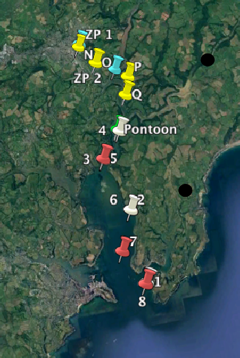
The addition of both nitrate and phosphate occurs at the same station of salinity 18.5 at 50˚15’34.56’’N, 005˚2’45.60’’W. Looking at the position of this station on a map, it is high up the Truro river (see map). The station is at a point in the river surrounded by a highly built up area, and so the inputs of phosphate and nitrate are likely due anthropogenic industrial activity or sewage effluent. Sewage effluent would explain the more evident input of phosphate, as it can account for almost 50% of the phosphate inputs into rivers (David and Gentry, 2000). A major sewage leaked occurred in the Truro river at Calenick Creek, a little further down river in 2015 (Gov.uk., 2017), inputting nutrients into the system- a similar event may have occurred here explaining the addition of nitrate and phosphate.
Silicate also behaves non-conservatively within the estuary (Figure 10), the highest concentration is at the river endmember of 147.2 mmol/L, and then all points fall below the TDL from a salinity of 13.78 onwards suggesting removal from the estuary until reaching the salt water endmember. This is most likely due to diatoms or other phytoplankton such as radiolarians utilising the silica to build their frustules and therefore lowering the concentration in the estuary.
All of the estuarine mixing diagrams are plotted with data (apart from the river endmember) only between salinities of 14 to 35.1, and so are lacking data from the upper estuary. This should be considered when drawing conclusions from the data, as behavior of the nutrients within the estuary from the mixing diagram may be inaccurate due to missing data from the upper estuary.


Figure 7: Richardson Number (Ri) profile for Station 5 in the Fal Estuary
Figure 9: Estuarine mixing diagram of salinity against phosphate concentrations (µmol/litre) for samples collected from the Fal estuary indicated by black circles. Blue dashed line indicates the theoretical dilution line, drawn between the river end-member concentration (salinity=0) and the point of highest salinity (35.1).
Figure 10: Estuarine mixing diagram of salinity against silicate concentrations (µmol/litre) for samples collected from the Fal estuary indicated by black circles. Blue dashed line indicates the theoretical dilution line, drawn between the river end-member concentration (salinity=0) and the point of highest salinity (35.1).
Figure 8: Estuarine mixing diagram of salinity against nitrate concentrations (µmol/litre) for samples collected from the Fal estuary indicated by black circles. Blue dashed line indicates the theoretical dilution line, drawn between the river end-member concentration (salinity=0) and the point of highest salinity (35.1).
Nutrient Depth Profiles
All nutrient depth profiles show a typical profile at each station that reflects their position in the estuary. For phosphate (Figure 11), nitrate (Figure 12) and silicate (Figure 13), at station 1 and 8 a uniform concentration is observed with depth, as these were positioned at the mouth of the estuary where tidal mixing leads to a fairly homogenous water column. Stations 2 and 7 which are slightly further in the estuary show higher concentrations at the surface which then decrease with depth, with this pattern following as the stations move up the estuary nearer to the river source. Statins 4 and 5, furthest up river have the highest surface concentrations for each nutrient (Station 5 0.75 mmol, 4.5mmol and 8.6 mmol and station 4 0.6 mmol, 4.4 mmol and 6.2 mmol for phosphate, silicate and nitrate respectively), which then decrease rapidly to a depth of 5m and then continue to decrease steadily with depth. The decrease with depth in the upper estuary can most likely be attributed to the stratification of water within the Fal estuary. As can be seen from Figure 3 salinity increases with depth, and temperature decreases (Figure 4). The warmer, fresher riverine water is less dense and so rests on top of the colder, more saline, and therefore denser seawater. The difference in densities preventing mixing, so the river water, rich in nutrients from weathering remains at the surface causing the higher concentrations of nutrients. This is confirmed from the calculation of the Richardson number of the upper estuary (Figure 7), indicating two water masses of turbulent flow, separate by a period of stability at 5.5m- the depth below which nutrient concentration start to decrease.


Figure 11: Depth profile of phosphate concentrations (µmol/litre) taken in the Fal estuary at Station 1(50˚8’42.96’’N, 005˚1’22.86’’W) Station 2(50˚10’42.18’’N, 005˚1’35.46’’W) Station 3(50˚12’11.10’’N, 005˚2’24.66’’W) Station 4(50˚12’54.42’’N, 005˚1’33.42’’W) Station 5(50˚12’12.48’’N, 005˚2’25.44’’W) Station 6(50˚10’42.16’’N, 005˚1’34.94’’W) Station 7(50˚9’37.68’’N, 005˚2’11.88’’W) Station 8(50˚8’40.28’’N, 005˚1’26.60’’W)
Figure 12: Depth profile of nitrate concentrations (µmol/litre) taken in the Fal estuary at Station 1(50˚8’42.96’’N, 005˚1’22.86’’W) Station 2(50˚10’42.18’’N, 005˚1’35.46’’W) Station 3(50˚12’11.10’’N, 005˚2’24.66’’W) Station 4(50˚12’54.42’’N, 005˚1’33.42’’W) Station 5(50˚12’12.48’’N, 005˚2’25.44’’W) Station 6(50˚10’42.16’’N, 005˚1’34.94’’W) Station 7(50˚9’37.68’’N, 005˚2’11.88’’W) Station 8(50˚8’40.28’’N, 005˚1’26.60’’W)
Figure 13: Depth profile of silicate concentrations (µmol/litre) taken in the Fal estuary at Station 1(50˚8’42.96’’N, 005˚1’22.86’’W) Station 2(50˚10’42.18’’N, 005˚1’35.46’’W) Station 3(50˚12’11.10’’N, 005˚2’24.66’’W) Station 4(50˚12’54.42’’N, 005˚1’33.42’’W) Station 5(50˚12’12.48’’N, 005˚2’25.44’’W) Station 6(50˚10’42.16’’N, 005˚1’34.94’’W) Station 7(50˚9’37.68’’N, 005˚2’11.88’’W) Station 8(50˚8’40.28’’N, 005˚1’26.60’’W)


Nitrate and Silicate sampled being processed in the Laboratory
Chlorophyll
Method
At each station in the estuary a vertical profile was taken to distinguish chlorophyll concentration at varying depths and to build up a horizontal transect along the estuary. Chlorophyll was measured from filtered samples of the water column at depths up to 30m using a Niskin Bottle attached to a rosette. The sample was filtered through a filterhead on a 50ml pipette and the filter was then submerged in 6ml of 90% acetone sample. The samples were transferred to a freezer and stored for 12 hours in a dark environment.
Results
The concentration of chlorophyll increased at each station as the transect
continued towards the mouth of the estuary with more saline waters (chlorophyll depth
profile). The tide was ebbing for the duration of the transect so the Conway followed
the retreat of the saline waters. At Station 1 the chlorophyll value was lowest at
0.018 ug/L at 30.06m depth. The highest reading at Station 8 was recorded as 1.284
ug/L at a depth of 25m. These values increase as depth decreases, at Station 1 chlorophyll
is recorded as 0.030 ug/L and at Station 8 surface readings are much greater at 2.2
ug/L.
The horizontal variations in chlorophyll concentration could affect plankton distrubtion along the Fal estuary.
Oxygen
Method
Glass bottles were filled with water collected from the Niskin bottles from the deepest depth measured. When filling the bottles, the tube was pushed to the base of the bottle to reduce bubble formation, and bottles were filled to the top so there was a rise in water. 1mL of Manganese Sulphate (a pink reagant) was added, followed by 1mL of Alkaline Iodide (clear reagant) and a cream precipitate was formed. The bottles were carefully sealed to prevent the oxygen escaping and submerged in a bucket of water. To minimise interaction between air and water the process was completed quickly.
Results
The dissolved oxygen concentration decreased with each station closer to the
mouth of the estuary. Estuaries are highly productive and have a high concentration
of nutrients, meaning there are less limits on photosynthesis and therefore allowing
higher rates. Additionally there are more marine organisms at the mouth of the estuary,
leading to increased levels of respiration, using up more oxygen than further up
the estuary. Net respiration takes place below the compensation depth and net photosynthesis
occurs above this depth. By studying the T/S diagram the stratified layers are clear
and indicate the thermocline. The samples were taken below the euphotic zone which
is where net repsiration occurs. Dissolved oxygen is influenced by temperature and
salinity as when sea surface temperature is high, oxygen saturation decreases. Bunsen’s
solubility curve demonstrates this physical phenomenon of gases.


Figure 14Vertical profile of Chlorophyll concentration (ug/L) at 8 Stations on Fal Estuary. Station 1(50˚8’42.96’’N, 005˚1’22.86’’W) Station 2(50˚10’42.18’’N, 005˚1’35.46’’W) Station 3(50˚12’11.10’’N, 005˚2’24.66’’W) Station 4(50˚12’54.42’’N, 005˚1’33.42’’W) Station 5(50˚12’12.48’’N, 005˚2’25.44’’W) Station 6(50˚10’42.16’’N, 005˚1’34.94’’W
Figure 15: Vertical profile of Percentage Oxygen Saturation at 8 Stations on Fal Estuary. Station 1(50˚8’42.96’’N, 005˚1’22.86’’W) Station 2(50˚10’42.18’’N, 005˚1’35.46’’W) Station 3(50˚12’11.10’’N, 005˚2’24.66’’W) Station 4(50˚12’54.42’’N, 005˚1’33.42’’W) Station 5(50˚12’12.48’’N, 005˚2’25.44’’W) Station 6(50˚10’42.16’’N, 005˚1’34.94’’W
The total abundance of phytoplankton was highly variable as the distance down the estuary increased, ranging from 150,000 cells/L at station 7 to 1,340,010 cells/L at station 5. Generally, the total abundance of phytoplankton was lowest at stations with intermediate salinities, whereas in high or low salinities the abundance was higher, but this is not true for station 7. Some phytoplankton species were only present in certain stations, most notably Cylindrotheca in station N and Chaetoceros in station Q. Ciliates were present in the upper and mid estuary, abundance peaked at 20000 cells/L at station, but were not present in the lower estuary. In stations N – 5 the phytoplankton communities were dominated by one or two species, whereas in station 7 the relatively small community consisted of many species with similar abundances. Interestingly, Nitzschia longissima was present in both station O in the upper estuary and station 5 in the lower estuary, but not stations P and Q in the mid estuary.
Certain species were closely associated with particular areas of the estuary: Cylindrotheca in the oligohaline and Chaetoceros in the mesohaline. Salinity does closely correlates with changes in species composition (Cox, 1977), but experimental work suggests that it may not be the only important variable (Admiraal et al. 1984). There is some suggestion that the population densities of some phytoplankton species are significantly related to a combined nutrient and salinity gradient (Underwood et al. 1998) This suggests that Cylindrotheca is adapted to high nutrient concentration and low salinity environment, and Chaetoceros is adapted to an intermediate nutrient concentration and intermediate salinity environment. Ciliate estuarine distribution is not directly related to tidal change or fluctuations in temperature and salinity as it depends on the availability of food (Webb, 1956), thus the high ciliate abundance in stations P and O may be due to high algal biomass caused by anthropogenic nutrient inputs. Station 7 may have low abundance because the low nutrient concentration limits production, causing the loss rates to exceed production rates (Hecky and Kilham, 1988).
Phytoplankton

Figure 16: Abundance of phytoplankton taxa in the Fal estuary in samples collected from 1m depth along a transect from 50 15’29’N 005 02’46’W to lat 50 9' 37.68''N long 005 2' 11.88''W . Samples were collected on 03/07/2017 on Winnie the Pooh (Stations N, O, P &Q) and RV Bill Conway (Station 5 & 7). Station samples are shown as columns and the species composition of the phytoplankton communities are depicted by the proportion of colours within the column. The time of sampling is shown above the columns in UTC.

Zooplankton
Total abundance increased with increasing distance downstream and zooplankton communities show clear zonation through the estuary. Mysidacae was only present in the lower estuary and decapoda larvae range was restricted to the mid estuary. Hydromedusae was the only zooplankton taxa recorded in the upper estuary and was also present at every station, the highest abundance recorded for hydromedusae was in the upper-mid estuary. Copepoda nauplii and copepoda were both present in the mid and lower estuary and the abundances of both peaked in the lower estuary, both constituting >30% of total abundance. Copepoda was more abundant in the mid estuary than copepoda nauplii, constituting >50% of the mid-lower estuary sample. Overall, copepoda was the most abundant zooplankton recorded throughout the estuary.
Zooplankton population maintenance depends on growth and behavioural responses offsetting the effects of physical processes, such as tidal currents, which remove the population from the estuary (Barlow, 1955). Physiological tolerance and flexibility to osmotic stress is a major factor influencing the survival of zooplankton. Mysidacae was restricted to the lower estuary which suggests it is adapted to high salinities, whilst hydromedusae was present throughout the estuary suggesting it is tolerant to a wide range of salinities. The peak of hydromedusae abundance in the upper-mid estuary suggests that that is its preferred zone where it displays optimal physiological performance. The distribution of copepoda and copepoda nauplii suggests that it is adapted to higher salinity environments, but is also very tolerant (Anger, 2003). The classification ‘copepoda’ contains many species, each with various specific tolerances to salinity (Lance, 1963) and so the taxa shows a wide distribution throughout the estuary. The copepoda are more tolerant to lower salinities than copepoda nauplii (Chinnery and Williams, 2004). In addition to this, nauplii have reduced swimming capability (Villante et al. 1993) and cannot maintain position in the estuary using behavioural responses, so would be advected into the lower estuary by tidal currents and river flow (Chinnery and Williams, 2004).
Figure 17: Abundance of zooplankton taxa in the Fal estuary in samples collected from 1m depth along a transect from 50 15’32’’N 005 2’44’W to 50 8’49.92’’N 005 1’ 30.42’’W. Samples were collected on 03/07/2017 on Winnie the Pooh (time 11:50 & 12:22) and RV Bill Conway (time 13:10 and 15:40). Station samples are shown as columns and the species composition of the phytoplankton communities are depicted by the proportion of colours within the column.
References
Admiraal, W., Peletier, H. and Brouwer, T., 1984, The seasonal succession patterns of diatom species on an intertidal mudflat: an experimental analysis., Oikos, 42, 30 – 40.
Anger, K., 2003, Salinity as a key parameter in the larval biology of decapod crustaceans., Invertebrate reproduction & development, 43, 29 – 45.
Barlow, J. P., 1955, Physical and biological processes determining the distribution of zooplankton in a tidal estuary., The Biological Bulletin, 109, 211 – 225.
Chinnery, F. E. and Williams, J. A., 2004, The influence of temperature and salinity on Acartia (Copepoda: Calanoida) nauplii survival., Marine Biology, 145, 733 – 738.
Cox, E. J., 1977, The distribution of tube-dwelling diatom species in the Severn estuary., Journal of the Marine Biological Association United Kingdom, 57, 19 – 27.
David, M. and Gentry, L., 2000, Anthropogenic Inputs of Nitrogen and Phosphorus and Riverine Export for Illinois, USA., Journal of Environment Quality, 29, 494.
Gov.uk., 2017, South West Water prosecuted for crude sewage spill in Truro River - GOV.UK. [online] Available at: https://www.gov.uk/government/news/south-west-water-prosecuted-for-crude-sewage-spill-in-truro-river [Accessed 10 Jul. 2017].
Hecky, R. E. and Kilham, P., 1988, Nutrient limitation of phytoplankton in freshwater
marine environments: A review of recent evidence on the effects of enrichment., Limnology and Oceanography, 33, 796 – 822.
Lance, J., 1963, The salinity tolerance of some estuarine planktonic copepods., Limnology and Oceanography, 8, 440 – 449.
Underwood, G. J. C., Phillips, J. and Saunders, K., 1998, Distribution of estuarine benthic diatom species along salinity and nutrient gradients., European Journal of Phycology, 33, 173 – 183.
Villante, F., Ruiz, A. and Franco, J.,1993, Summer zonation and development of zooplankton populations within a shallow mesotidal system: the estuary of Mundaka., Cahiers de Biologie Marine, 34, 131 – 143.
Webb, M. G., 1956, An Ecological Study of Brackish Water Ciliates., Journal of Animal Ecology, 25, 148 – 175.
DISCLAIMER: The findings and views expressed on this website are not those of the University of Southampton or the National Oceanography Centre