Home Offshore Estuary Pontoon Habitat Mapping Index

Physics & Chemistry

Chemistry analysis

Estuarine mixing diagrams are primarily used to indicate the extent of physical mixing of fresh and saline waters of different compositions along salinity gradients. If there are no biogeochemical processes occurring within the estuary then mixing results in a linear relationship between the two endmembers, this is known as a theoretical dilution line (TDL) (Chester, 2000).

Mixing diagrams assume that the estuary is in a steady state, there is only one freshwater and one saline endmember and that the concentration of the endmembers is constant on a timescale greater than the residence time of the water in the estuary. They also assume that there are no additional inputs. The River Allen was used as the freshwater endmember, whilst the Fal estuary has six main tributaries and 28 minor creeks it can be assumed that these have a negligible influence on the nutrient concentrations and mixing of fresh and saline water within the estuary (Langston et al., 2003).

Figures 8 - 10 show the mixing diagrams for three major nutrients required for phytoplankton growth: silicon, nitrate and phosphate. (James, 2005). Group 1 data is in red and Group 2 data is in green. The nutrient concentrations from Bill Conway samples are clustered together on the mixing diagrams whereas the Winnie the Pooh samples are spread out along a larger salinity gradient as the boat was able to sample further up the estuary.   

Silicon appears to behave non-conservatively, with slight removal observed in the upper estuary from the Winnie the Pooh samples. This is likely due to the high presence of diatoms (Cylindrothica closterium) that remove silicon from the water column for frustrule formation. Silicon occurs in high concentrations in the upper estuary (River Allen endmembers) as 99% of silicates in rivers are a product of chemical weathering of silicate bearing catchment bedrock. The bedrock in this region is primarily granite.

For phosphate non-conservative behaviour is observed, the Winnie the Pooh samples lie above the TDL showing that there is addition to the system. Whilst mixing diagrams can’t be used to exclusively show the cause of this addition it is most likely due to Station Q being situated near a sewage treatment works. Sewage plants are associated with high phosphate concentrations, so act as an additional source of phosphate to the estuary. The other Winnie the Pooh samples also show phosphate addition, likely due to the ebbing tide causing down estuary movement of phosphate concentrations (low water was at 09:41 UTC on 06/07/17) (UK Hydrographic Office, 2017).

Nitrate behaved conservatively this is due to non-conservative behaviour only being observed if nitrate has a long residence time. So any removal by phytoplankton is masked by a high input rate from the River Allen.

CTD Profile Analysis

CTD profiles were taken at four stations in the lower estuary (Stations 18-21). At each station an Acoustic Doppler Current Profile (ADCP) transect was taken across the estuary as well as when CTD measurements were being taken. At the start of the study the tide was flooding as low water was at 09:41 UTC. The first three ADCP transects were taken at 12:44, 13:10 and 14:13 UTC respectively and show the tide was flooding.

On the turn of the tide three ADCP transects were taken to form a triangle to observe the water movement. The triangle shows that the tide was still flooding in the centre of the channel however it had begun to ebb along the banks of the estuary. This can be seen by the East-West Transect and the South West-North East and North West-South East transects in figure 2.

At all four stations the phosphate concentration was significantly lower than the silicon and nitrate concentrations. The fine structure of the nutrient profiles with depth is lost as sampling was only taken at the surface and bottom of the water column as well as at a mid-depth. Down estuary at Stations 19-21 a clear thermocline and halocline is present at around 5 m.

Station 18: 50 12.176 N, 005 002.411 W. 12:36 UTC

Station 18 was situated at 50 12.176 N, 005 002.411W as seen in Figure 2. ADCP measurements show that the fastest flow occurred at depth near the seabed. (Figure 14).

The water column is stratified with warm, less dense freshwater overlying denser, cooler saline water. This is typical for an estuarine environment. There are two peaks in fluorescence, one between 4-7 m in the freshwater layer and another between 8-12 m. The Richardson (Ri) number is a comparison of the stabilising forces of density stratification to the destabilising forces of velocity shear (Dyer, 1997). It is used to determine if the flow is turbulent or laminar in the vertical picture. At 4 m the Ri number is greater than 1 indicating laminar flow, this roughly corresponds with the thermocline between the stratified warm fresh water and cooler more saline water at depth. Within the two separate layers of water the Ri indicates turbulent flow and hence mixing, where fluorescence peaked.

Fluorescence peaked at 4-7 m, water samples taken at 5.6 m and 13.7 m reveal that the chlorophyll concentration was 0.5 (µg/L) at both depths so it can’t be concluded that the peak in fluorescence is due to high amounts of phytoplankton at this depth. However, Holm-Hansen et al. (1965) have shown a direct relationship between chlorophyll concentration and fluorescence. This is supported by nitrate and phosphate concentrations both decreasing from the surface to 5.6 m suggesting a phytoplankton bloom between 4-8 m and subsequent uptake of these nutrients. Below this depth nitrate and phosphate concentration both increase again. Silicon behaved oppositely to nitrate and phosphate, increasing from the surface to 5.6 m and then decreasing again.

Station 19: 50 11.452N, 005 002.755 W. 13:42 UTC

Station 19 was situated at 50 11.452 N, 005 002.755 W as seen in Figure 2. ADCP measurements combined with the CTD profile shows that there was a layer of fast flowing warm less saline water between 1-6 m (Figure 18). An Ri of 10 at 2 m shows that the freshwater layer was moving as very laminar flow. Below 3 m the water column behaved as turbulent flow (except at 10 m), this is due to stratification.

There was a distinct thermocline and halocline at around 5 m, resulting in a highly stratified surface layer and a well-mixed bottom layer of water, which varies little with depth due to turbulent mixing. Hence why phosphate concentration remained fairly constant with depth and fluorescence only slightly increased. Overall silicon concentrations decreased with depth and nitrate concentrations increase with depth. At 3 m (within the freshwater layer) there was an increase in nitrate concentration and a decrease in silicon concentration. This is due to the freshwater input providing a high nitrate concentration, resulting in rapid removal of silicon from the water column by diatoms (Lewin, 1955).

Station 20: 50 10.741 N, 005 001.603 W. 14:03 UTC

Station 20 was situated at 50 10.741 N, 005 001.603 W as seen in Figure 2. ADCP measurements show that the fastest flow occurred at depth near the seabed. (Figure 21).

Like station 19 there was a distinct thermocline and halocline at around 5 m, resulting in a highly stratified surface layer and a well-mixed bottom layer of water, which varies little with depth. Phosphate and chlorophyll concentration remained fairly constant with depth and fluorescence slightly increased. Overall silicon concentrations decreased with depth and nitrate concentrations increased with depth (this is the opposite to what was observed at station 19). At 11 m the silicon and nitrate concentrations were similar.

Station 21: 50 08.666N, 005 01.435W. 14:52 UTC

Station 21 was situated at 50 08.666 N, 005 01.435 W as seen in Figure 2. ADCP measurements show that flow remained fairly constant with depth. ADCP transect 4 shows that the tide was beginning to turn as it was still flooding in the centre of the channel where the station was situated but had started to ebb along the banks of the estuary (Figure 25).

Like stations 19 and 20 there was a distinct thermocline and halocline at around 5 m, with phosphate concentration remaining fairly constant with depth. Fluorescence increased with depth until around 12 m and then remained fairly constant, this coincided with an increase in chlorophyll concentration from 1.0-2.4 (µg/L) and a decrease in nitrate and silicon concentrations between the surface and 12.8 m. This is due to high abundance of phytoplankton at this depth resulting in the uptake of nitrate and silicon from the water column.

At the surface there was a layer of warm saline water overlying cold fresh water; since this is still an estuarine environment, it is expected that cool fresh water would be at the surface. As the station was situated in the mouth of the estuary near Black Rock, this feature could be due to the incoming flood tide trapping fresh water into surrounding bays at the mouth of the estuary. The CTD was taken on the turn of the tide as observed in Figures 2d - 2f (high tide occurred at 15:36 UTC). The turn of the tide at high water results in eddy systems, drawing in the fresh water from the bays causing mixing. This is indicated by the Ri number which is less than 0.25 suggesting that the water column was undergoing turbulent mixing. The mixing causes the unusual characteristics shown in the graph. Here, temperature dominates stability as there is a 2OC temperature gradient between the surface and deep water, and only a salinity gradient of 0.2, which has much less effect on the water.

Introduction

The aim of the estuary practical was to look at the variation of nutrients with varying salinities along the whole estuarine system in the River Fal.

The experimentation on the river was split between two boats. The Winnie the Pooh collected the shallow estuary data from The King Harry Ferry (50°21.63N, 5°02.66W), up past Malpas towards Truro (50°14.96N, 5°02.20W). RV Bill Conway was used to survey the deeper part of the channel from The King Harry Ferry up to the mouth of the Estuary at Black Rock (50°14.52N, 5°02.85W). ADCP transects were taken across the estuary at points where other riverine inputs were flowing into the main Estuarine Channel. (See Figure 2).

Methods

Niskin Bottle Deployment

A horizontal niskin bottle was deployed off the side of the boat and a sample was taken approximately 30cm beneath the water’s surface by dropping the weight on the closing mechanism. The sample was brought to the surface, then the water used to rinse the probe and two sample containers. The containers were then used to collect two samples, one for chemistry preparation and the other was used with the probe to record pH, temperature and salinity at each location, before being filtered for chlorophyll preparation.

Chlorophyll Preparation

The sample was filtered through a glass fibre filter for each station, and the filter was then added to 6ml of 90% acetone. This was repeated 3 times for each station and the tubes were inverted ready to chlorophyll analysis back in the lab.

The vile numbers and corresponding locations were recorded.

Chemistry lab methods

Chlorophyll a sample processing

The chlorophyll a samples collected off the Pontoon, Winnie the Pooh & Bill Conway on 06/07/2017 and were processed on 07/07/2017 using a fluorometer. The fluorometer was used to calculate the chlorophyll a concentration in the water samples by generating a reading based on the fluorescence of the sample. This reading (µg/L) was recorded and inputted into an excel spreadsheet that includes an equation multiplying the water sample fluorescence readings by the volume of acetone used (6 ml) over the volume of sea water (50 ml). The end result of this equation gave the chlorophyll a concentration in the water samples (µg/L).

Nutrient & oxygen sample processing
The concentrations of nutrients & oxygen were calculated using standard methodology:
Phosphate and Silicate: Parsons et al.,1984.
Oxygen: Grasshof et al., 1999.
Nitrate (by flow injection analysis): Johnson et al.,1984.

Biology

Zooplankton

Zooplankton composition is heavily copepod dominated in the upper, less saline, parts of the estuary. In the mouth of the estuary by Black Rock the zooplankton has a mixed population ofCladocera, Hydromedusae and Copepoda. A variety of other species were also found in low abundance (see Pie Charts). It is to be expected with the increased nutrients from riverine input. The lack of fish larvae indicated that the nutrient rich estuary is not being used as a nursery ground for the early life stages of fish. This could be due to poor water quality which is low in nitrate and phosphate along the whole estuary.

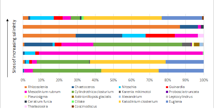
Phytoplankton

There is a greater abundance of phytoplankton in the fresher water located further up the estuary. This is likely due to the increased input of nutrients at this location, in conjunction with there being greater light availability here, as these favourable conditions are able to support heightened planktonic growth. Mesodinium rubrum is a species that was continually present along the range of salinities, this is concurrent with the knowledge of this species as it is a euryhaline. The greatest population of rubrum was found in the mid salinities. Katodinium closterium was only found in high salinity water, with large abundance. The indication is that closterium is also a euryhaline but is outcompeted in the mid-range salinities by stenohalines but can then thrive at the extreme salinities. An alternative explanation for the variations in abundance of the phytoplankton could be that the water was shallower in the heights of the estuary. This means that the water samples were taken closer to the surface where there is greater light availability. Abnormalities in the quality of phytoplankton identification could explain the differing distributions of phytoplankton, with various different scientists processing the samples.

Disclaimer: All the opinions expressed in this site are that of Group 2 and not necessarily the University of Southampton or the National Oceanography Centre.

Click charts to enlarge

Estuary

Conway

Winnie the Pooh

Click charts to enlarge

Figure 1 a): Stars at which points a CTD and Niskin Bottle Rosette were deployed in the Fal Estuary on 06/07/17 off the back of R.V. Bill Conway.

Figure 1b): Points indicting where water samples were taken in upper Fal Estuary and Truro River on vessel Winnie the Pooh.

Figure 2: Green Pins represent the start of an ADCP Transect across the estuary. Red indicates the end point. The Point Markers are the track of zooplankton net trawls in the upper estuary and across the mouth of the estuary. The pink triangle shows the track of the ADCP around the mouth of the Percuil River to the East, the Carrick Roads to the South and the remaining rivers to the North West.

Click on transect lines to view ADCP ship tracks & contour plots.

Chemistry Preparation

Lugol’s bottles

100ml of the sample was measured out using a syringe and measuring cylinder, previously rinsed out using the sample water. The 100ml is then added to a lugol’s bottle containing iodine, which stains the phytoplankton within the bottle.

Silicon bottles

100ml of the sample is measured out using a syringe and measuring cylinder and filtered. The bottle is then rinsed in the filtered sample, and 100ml is added to the plastic bottle.

Phosphorous/Nitrate bottles

100ml of the sample is measured out using a syringe and measuring cylinder and filtered. The bottle is then rinsed in the filtered sample, and 100ml is added to the plastic bottle.

The numbers of all the bottles and the stations they correspond to were recorded.

How we chose our Winnie the Pooh stations

The tides were important when considering our locations. Since we experienced low tide when on the boat (at 9:40 UTC), it was not possible to go further than Malpas until later in the day, therefore, we chose to take the first sample at Malpas, where the salinity was as low as we could currently reach, then heading back downstream, two samples were taken equidistant apart, being careful not to sample too close to tributaries entering the river system which would distort the data. At approximately 11:00 UTC, we headed as far upstream as possible and sampled there, finding a salinity of 25.95. Here, however, there were other inputs which needed to be considered during analysis, such as the sewage treatment input.

Click charts to enlarge

Click charts to enlarge

Click charts to enlarge

Click charts to enlarge

Click charts to enlarge