ESTUARY

Contents

Information

Back To Top

DISCLAIMER: The words and views expressed here solely represent the findings made by this group and by no means those of the University of Southampton.

Date: 28th June 2016

Time (GMT): 07:00 to 12:11

Low Tides (GMT): 04:59, 17:27

High Tides (GMT): 10:59

Tidal Range: 3.19m

Weather Conditions: 8/8ths cloud cover (07:17 GMT), windy, 3.2m/s wind speed, wind direction 168°, moderate rainfall at 10:14 GMT, wind speed increased to 7.8m/s at 11:05 GMT

• Introduction

• Methods

• Results

• Discussion

• Summary

• References

Introduction

Sampling in the Fal Estuary was carried out onboard RV Bill Conway on 27/6/16 between 07:00 and 13:00 GMT.

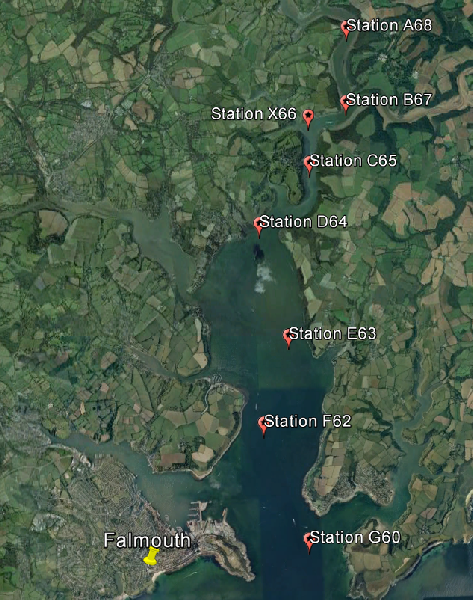
The aim of the survey was to investigate how chemical, physical and biological properties vary spatially along the estuary. This region where freshwater meets seawater provides an environment where conditions can change in a short space of time, giving information about the processes occurring. The locations of the eight sampling sites were determined prior to the survey, extending up the estuary from Black Rock at the mouth.

Methods

The same field methodology was used as on RV Callista for the offshore practical. At each station a CTD profile was taken to examine the water column structure, which was then investigated accordingly. ADCP data was also taken in order to calculate the Richardson Number (Ri), which describes how the stability of the water column varied along the estuary.

Only a small number of samples for dissolved oxygen and phytoplankton could be taken due a limited number of sample bottles available.

A Secchi disk was used to describe how the depth of the euphotic zone varied along the estuary.

Sampling was repeated at the Black Rock site (G60 and G61) because the initial data logsheet was lost overboard.

Similarly, the same laboratory analysis was used as from the offshore practical. There were issues with the U1800 fluorometer, which required recalibrating after each sample. This may have affected the accuracy of results taken.

Results

Discussion

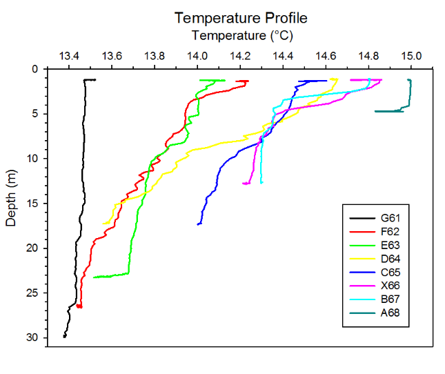
Water temperature increased with distance from the mouth of the Fal estuary (Figure 9). Inversely, salinity decreased over the same distance (NOAA, 2016). This was due to the decreased influence of seawater and increased influence of freshwater, which was principally inputted by rivers, for example the Rivers Fal and Truro. At the mouth of the estuary (Station G61), water temperature and salinity were relatively high and low respectively. These parameters remained constant with depth at this location. This was the result of a large tidal influence and almost no river influence.  Conversely, stratification existed at approximately 3 m water depth for stations X66 and B67 because there was both a strong tidal and river influence. It should be noted that salinity was still relatively high at Station A68, the most upstream site, which indicates a significant tidal influence existed.

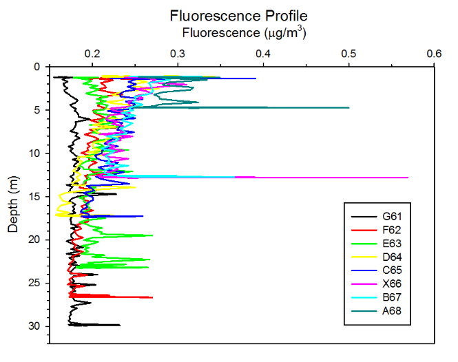
Fluorescence, generally, decreased with depth due to the attenuation of light (Figure 11). However, it is important to note that there is much noise in the data and the values are only relative because a chlorophyll calibration was not available. The attenuation of light increased with distance upstream as a result of increasing turbidity (Figures 11 & Brown, 1984). Figure x supports an increased turbidity as it shows that transmission was smaller at the upstream sites compared to the mouth of the estuary. This is because riverwater carries a greater suspended load as a result of erosive processes. The rapid increase in transmission at 10 m water depth at station D64 was likely the result of some external factor, such as a passing vessel.

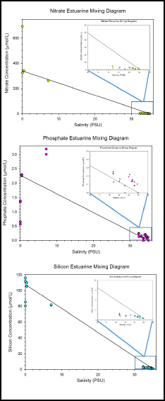
The concentrations of the three nutrients sampled are displayed in Figure 12. Nitrate and silicate both fall below the theoretical dilution line. This is evidence of non-conservative behaviour and removal during estuarine mixing. A diatom bloom would explain this pattern. Phytoplankton require nitrate for the formation of biomolecules, such as deoxyribose nucleic acid. Siliceous phytoplankton require silicate for the formation of frustules. On the other hand, phosphate was arranged above the theoretical dilution line, which suggests the element was added during estuarine mixing. Possible inputs of phosphate include sewage outfalls, agricultural run-off and natural processes that occur in neighbouring wetlands. Concentrations of all three nutrients were higher in the riverwater endmember compared to the seawater endmember. This was, again, due to high-suspended load carried by the riverwater.

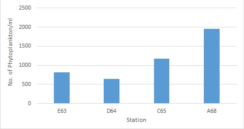
A positive correlation between phytoplankton abundance and distance from the mouth of the estuary existed. This was the result of higher nutrient concentrations upstream. Furthermore, these changes can also be linked to variation in zooplankton abundance (Aziz et al., 2006). Phytoplankton abundance was lowest at Station D64, which coincided with a peak in zooplankton abundance. Conversely, phytoplankton abundance was highest at Station A68. At this location, the zooplankton population was relatively small and dominated by a single phytoplankton group (copepods).  As a result, the number of feeding mechanisms will be limited leading to a reduced feeding efficiency.

References

• Brown, R. (1984). RELATIONSHIPS BETWEEN SUSPENDED SOLIDS, TURBIDITY, LIGHT ATTENUATION, AND ALGAL PRODUCTIVITY. Lake and Reservoir Management, [online] 1(1), pp.198-205. Available at: http://www.tandfonline.com/doi/pdf/10.1080/07438148409354510 [Accessed 1 Jul. 2016].

• Oceanservice.noaa.gov. (2016). NOAA's National Ocean Service Education: Estuaries. [online] Available at: http://oceanservice.noaa.gov/education/kits/estuaries/media/supp_estuar10c_salinity.html [Accessed 1 Jul. 2016].

• Aziz, N. E., Gharib, S. M., Dorgham, M. M. 2006. ‘The interaction between phytoplankton and zooplankton in a Lake-Sea connection, Alexandria, Egypt’, International Journal of Oceans and Oceanography, 1, pp. 151-165. Available at: http://connection.ebscohost.com/c/articles/21200634/interaction-between-phytoplankton-zooplankton-lake-sea-connection-alexandria-egypt [Assessed 1/7/2016]

Summary

Water temperature and turbidity increase as one moves up the estuary. On the other hand, salinity decreased over the same distance. There was evidence of both well-mixed and stratified water columns, which leads one to the conclusion that the Fal estuary is partially mixed. All three nutrients exhibited non-conservative behaviour and declined in concentration down the estuary. As a result, phytoplankton abundance similarly decreased.

Figure 2: a table of latitudes, longitudes and times for each site visited in the estuary.

ADCP Velocities

All stations have a homogenous velocity throughout the water column (eg Station G61; figure 4). This is an indication of a flood tide, as the entire water body is moving at a similar rate. Station C65 (figure 5) shows a different velocity contour graph. This is because there was an abandoned fishery in that area that could be acting as an obstacle for the flow to pass. From the ADCP data, we were able to determine the total velocity discharge (m3s-1) for each station. As we approached high water the velocity discharge decreased until at high water we recorded the lowest discharge (Station C65; figure 5). After this the discharge increased again (Station A68; figure 6).

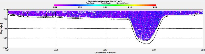
Figure 4: Station G61 transect velocities, total discharge = 3550m³/s

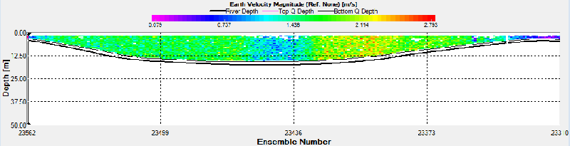
Figure 5: Station C65 transect velocities total discharge = 62.49m³/s

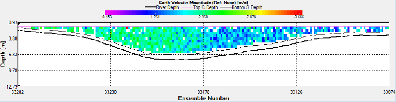
Figure 6: Station A68 transect velocities, total discharge = 197.79m³/s

Figure 3: map of different stations visited in Falmouth estuary.

(Click Picture To Enlarge)

(Click Picture To Enlarge)

(Click Picture To Enlarge)

(Click Picture To Enlarge)

(Click Picture To Enlarge)

Figure 7: changes in fluorescence in µg/m³ with respect to depth for various stations along the estuary.

Figure 8: changes in salinity (PSU) with depth across various estuarine stations.

Figure 9: changes in temperature (°c) with depth at various estuarine stations.

Figure 10: changes in transmission (V) with changes in depth across various estuarine stations.

Transmission

Transmission profiles from the eight sampling stations are represented in Figure x. Transmission was greater at stations G61-E63, which were located closest to the mouth of the Fal estuary, and there was little variation with depth. Transmission was lowest at Station A68, the most upstream site. Similarly, transmission did not change significantly with depth at this location. Transmission increased with depth at stations C65-B67. There was a rapid increase in transmission at Station D64 from 4.39 V at 5m depth to 4.47 V at 10m.

Salinity

The changes in salinity with depth are shown in Figure 8 Salinity remains relatively constant with depth at stations G61, F62, E63 and A68. Salinity increased significantly in the upper 5 m of the water column at stations X66 and B67. For example, at X66, salinity increased from 32.44 to 33.10 between the surface and 5 m water depth respectively. After this point, salinity varied little with further increases in depth. Salinity steadily increased with depth at stations D64 and C65.

Temperature

Figure 9 describes the temperature profiles of the eight survey stations. Water temperature remained relatively constant with depth at stations G61 and A68. A steady decline in water temperature with depth was observed at stations F62-C65. At stations X66 and B67, water temperature decreased sharply by approximately 0.4 °C to 14.35 °C over several metres to 5 m water depth. Temperature increases with distance from the mouth of the river.

Fluorescence

The fluorescence profiles from the eight sampling stations are displayed in Figure 7 Fluorescence, generally, decreased with depth from approximately 0.325 μg/m3 at the surface to 0.175 μg/m3 close to the seabed.

Nutrient Concentrations (Left)

The behaviour of nitrate, phosphate and silicate in the estuary is detailed in Figure 12. Nitrate and silicate results fall below the theoretical dilution line. In contrast, phosphate was arranged along the theoretical dilution line, with the exception of two data points at a salinity of approximately 8.

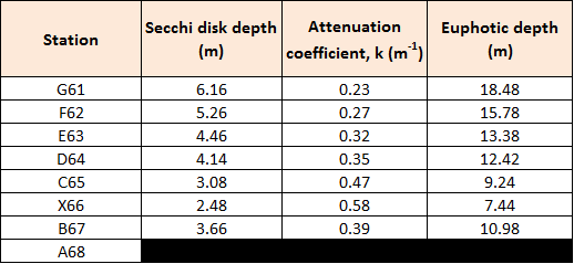
Figure 11: stations with respective secchi disk depths, and calculated attentuation coefficient (1.44/secchi disk depth in meters) and euphotic zone (3x secchi disk depth in meters). Data not available for Station A68 due to strong winds and currents.

(Click Picture To Enlarge)

(Click Picture To Open PDF In A New Tab)

The attenuation coefficient, generally, increased along the stations. Conversely, euphotic zone depth decreased with distance up the estuary.

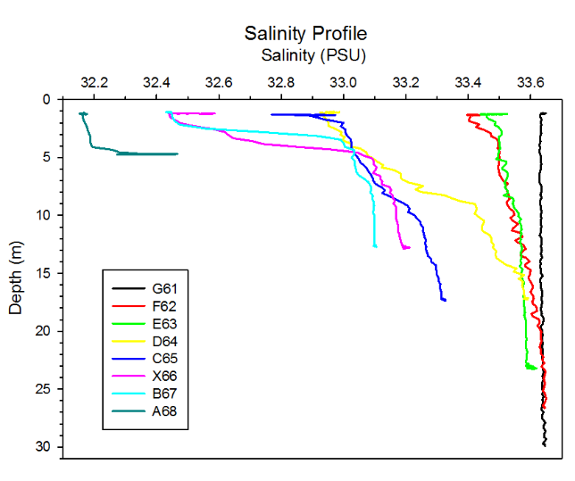
Figure 13: zooplankton abundance and dominant species per m³ at 3 stations: G61, D64 and A68.

Figure 14: phytoplankton abundance per ml at 4 stations: E63, D64, C65 and A68.

Figure 12: estuarine mixing diagrams for nitrate, phosphate and silicate.

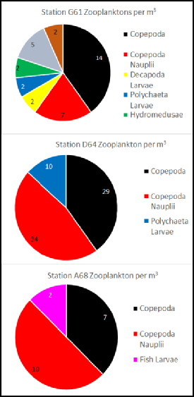
Zooplankton (Right)

Copepoda and Copepoda Nauplii accounted for the majority of zooplankton at the three stations. The zooplankton community at station G61 was relatively diverse and other groups such as  polychaete larvae were present. Zooplankton diversity was greatest at station D64 and lowest at station A68.

(Click Picture To Open PDF In A New Tab)

(Click Picture To Enlarge)

Phytoplankton

Phytoplankton abundance was lowest at station D64 and highest at station A68.