

Group 8 - Falmouth 2015
Offshore
With the use of the research vessel, Callista, between 07:56 UTC and 15:23 UTC we were able to sample the water column in an offshore environment. By deploying a CTD attached to a rosette, data was collected from chosen depths recording salinity, temperature, pressure, latitude, longitude, turbidity, irradiance, conductivity, density, fluorescence, depth and pressure. The rosette was deployed by using a winch and an a-frame. As well as the CTD being attached to the rosette, six niskin bottles were placed within the frame. The niskin bottles enable us to retrieve water samples from various depths. By sending down a messenger the niskin bottles close, capturing a sample in the water column at a specific depth. An ADCP was used giving us the velocity, back scatter and flow. The ADCP was attached to the underside of the vessel. Zooplankton samples were collected at multiple stations using a zooplankton net of 50cm diameter. The sample was collected through the water column by lifting the net up from a starting depth to an end depth. Upon recovering the niskin bottles back on deck, samples were prepared, ready for analysis in the lab.
The CTD was used to obtain data concerning the stratification of chlorophyll present within the water column.
Phytoplankton
Disclaimer; the views and opinions expressed are those of the individual and not necessarily those of the University. ©El Sharkke 2015

Zooplanton
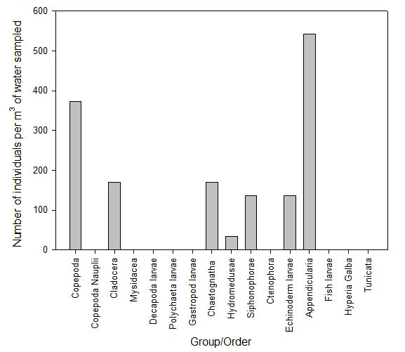
FIGURE X; Graph to show zooplankton groups and orders caught in net at offshore station 60 at depths 15-0m.
Figure X shows that the most abundant zooplankton species present in the offshore water sample taken by group 8 at station 60 at 15-0m was appendicularia at 550 individuals per m-3 of water sampled. This was followed by copepoda at 375 individuals per m-3 of water sampled. The least abundant species present was hydromedusae at around 40 individuals.
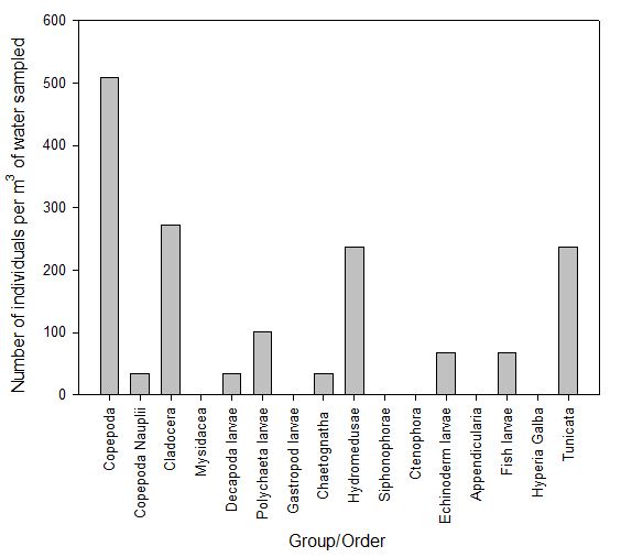
FIGURE X; Graph to show zooplankton groups and orders caught in net at offshore station 60 at depths 30-15m.
Figure X shows that copepods are extremely abundant at offshore sampling station 60 at depths of 30-15m with densities of around 510 individuals per m-3 of water sampled. Cladocera, hydromedusae and tunicata were present at densities of around 250 individuals per m-3. The least abundant species of zooplankton present in this sample were copepod nauplii, decapod larvae and chaetognaths at around 40 individuals per m-3 of water sampled.
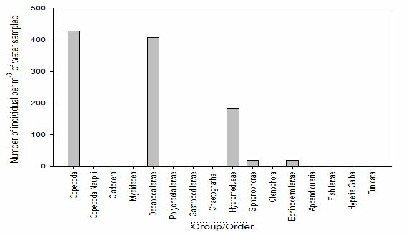
FIGURE X; Graph to show zooplankton groups and orders caught in net at offshore station 63 at depths 25-0m.
Figure X shows that the most abundant species of zooplankton at station 63 and depths of 25-0m was copepoda at densities of 430 individuals per m-3 of water sampled, closely followed by decapoda larvae at 410 individuals per m-3. The least abundant species that were present in this sample were siphonophores and echinoderm larvae, both at just 30 individuals per m-3 of water sampled.
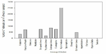
FIGURE X; Graph to show zooplankton groups and orders caught in net at offshore station 66 at depths 15-0m.
Figure X shows that the most abundant zooplankton in offshore sampling station 66, depth 15-0m was hydromedusae, at 2600 individuals per m-3 of water sampled. This was a lot higher than the numbers of any other species present, and was followed by gastropod larvae at only 875 individuals per m-3 of water sampled. The least abundant species present was polychaete larvae at just 250 individuals per m-3.
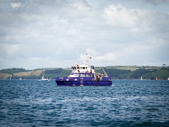
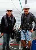
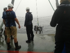
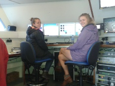
FIGURES 2, 3, 4, 5; (left to right) pictures showing (from left) R.V Callista, Sam and Richard with the rosette, the rosette being deployed and Katherine and Emily tracking the rosette depth, firing bottles and taking ADCP transects.
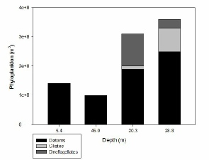
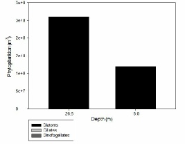
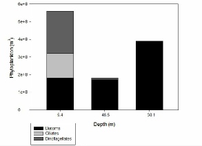
FIGURES 20, 21, 22 & *; phytoplankton graphs showing the composition of the phytoplankton communities at stations 60 (), 63 () and 66 () for different depths.
Figure X shows that at station 60 phytoplankton levels are highest at the sampling depth of 28.8 metres. The sampling depth with the lowest phytoplankton count at this station was 45 metres. Diatoms are most abundant at 28.8 metres and least abundant at 45 metres, whilst ciliates are also highest at 28.8 metres, followed by counts at 20.3 metres. They were absent at both of the other depths sampled. Dinoflagellates were also absent from the 5.4 and 45 metre sampling depths, however they were present in large numbers at 20.3 metres and somewhat abundant at 28.8 metres.
Figure X shows that at station 63 the sampling depth of 26.6 metres contained the highest densities of diatoms, with the 5 metre depth only having roughly half the amount of the former. All ciliates and dinoflagellates were absent at this station at both depths sampled.
Figure X shows that at station 66 diatoms were more than twice as abundant at depths of 30.1 metres than they were at 5.4 and 46.5 metres which both measured similarly low in diatom abundance. Ciliates were absent at all depths except 5.4 metres which accounted for a little under a third of the total phytoplankton count at this depth. Dinoflagellates were only present at depths of 5.4 and 46.5 metres, but were much more abundant in the shallower surface depths than they were nearer the seafloor.
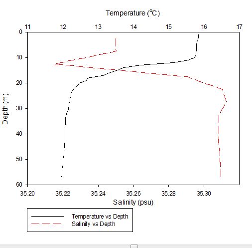
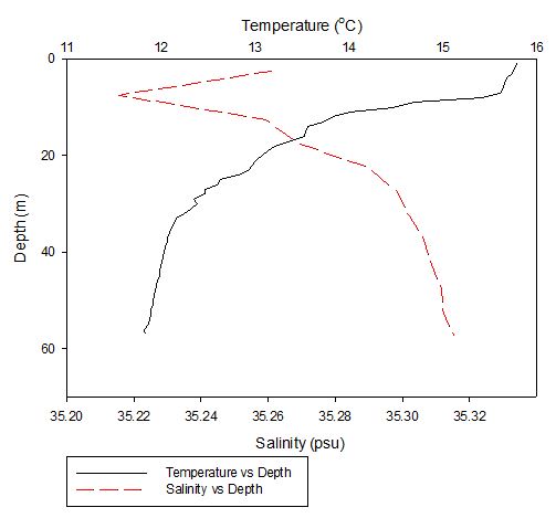
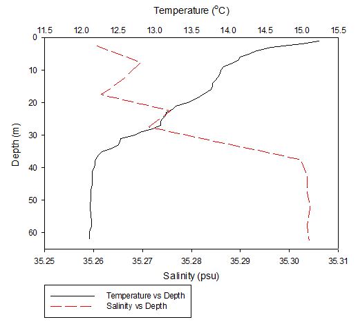
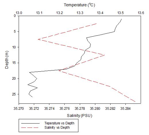
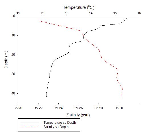
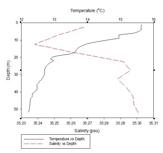
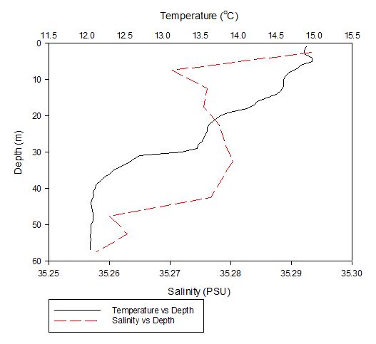
Temperature and Salinity
Temperature and salinity were measured using the CTD that was attached to the the rossette.
Richardson Number
The Richardson Number was calculated using salinity, temperature and depth from the CTD data to calculate density and the ADCP data to give current velocity with depth. The Richardson Number gives an indication of the type of flow and the subsequent mixing as a result. If Ri is >1 flow is laminar, <0.25 flow is turbulent, and 0.25-1 it is transitional between the two types of flow.
Dissolved Oxygen
The offshore data for dissolved oxygen is unusable. Some of the samples required an anomalously huge amount of Thiosulphate concentration before turning clear, the largest of which was 142ml The reason for this was human error during the titration. The titration was mechanically assisted and the machine that was used requires a refill button to be pressed after each sample. During the analysis this task wasn’t completed each time and the button wasn’t pressed. When this happens, the pipette automatically refills however the computer does not recognize this. As a result, less Thiosulphate was added to the sample than what was indicated on the screen. This explains the anomalous results we achieved in the samples.
Nutrients
Water samples were taken using niskin bottles attached to the rosette. Further analysis in labs was carried out to determine silicon nitrate and phosphate concentrations. Water samples were taken at three sites at different depths, The results are shown in the graphs below.
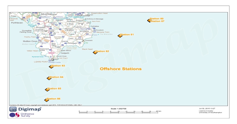
FIGURE 1; a map of Lizard Point and the surrounding area showing the exact locations of each sampling site.
Figure 1, taken closest to the estuary, clearly shows 2 water masses within the water column with both a thermocline and halocline separating them. As boat moves further away from the estuary the 2 water masses become less distinct as the water is gradually mixed. Figure 4 is taken directly off the coast of Lizard point. This is an area with large waves, coastal upwelling and lots of turbulence within the water column. As a result while there is a general pattern with a reduction in temperature and an increase in salinity with depth pockets of water within the water have different characteristics which leads to the lack of smoothness on the profiles. Off shore the profiles are much smoother and the water column is relatively well mixed. There is a gradual decrease in temperature creating a gentle thermocline.
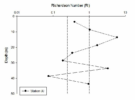
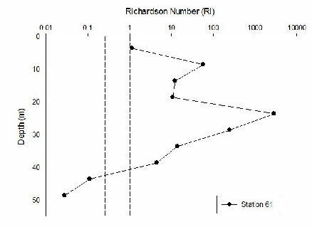
Station B (60) has laminar flow at all depths and so does Station 61 until 40m depth and below where flow becomes turbulent. As the transects and stations move further away from the coast there is a lot less laminar flow and increasing turbulence. For example Station 63 has turbulent flow below 15m. Station 66 has little laminar flow and mainly turbulent and transitional flow. Generally turbulence is high in deeper water and laminar flow in the surface waters and therefore no mixing.
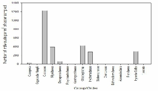
FIGURE X; Graph to show zooplankton groups and orders caught in net at offshore station 66 at depths 35-0m.
The most abundant zooplankton species present in the offshore water sample taken at station 66 at a depth of 35-0m was cladocera at 1250 individuals per m-3 of water sampled, picturised in figure X. The next abundant species was chaetognatha but at densities of only 440 individuals per m-3 of water sampled. The least abundant species was copepod at just 40 individuals per m-3 of water sampled, despite other similar stations having high counts of these.
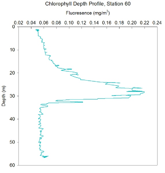
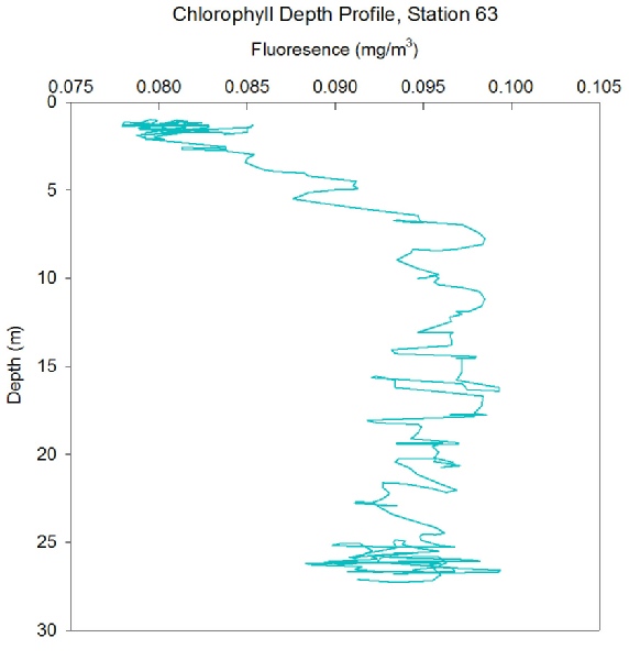
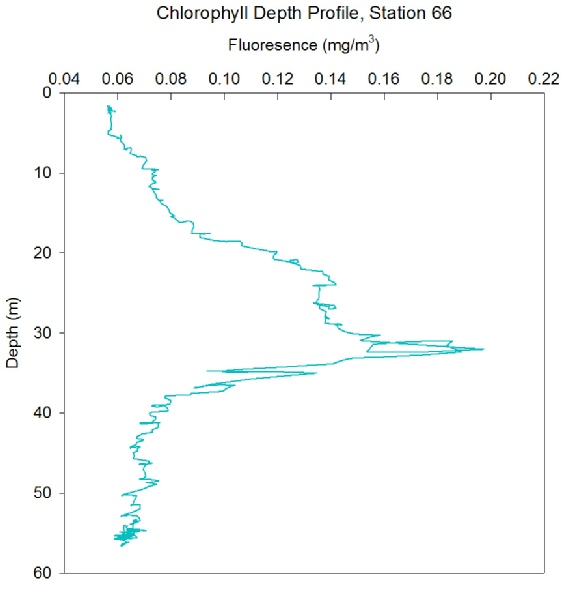
FIGURES 15, 16 and 17. Graphs showing chlorophyll with depth
Station 60 - Chlorophyll increases at a gradually faster rate with depth, with a fluorescence at the surface of 0.05 mg/m3, to a Chlorophyll maximum at a depth of around 27m, with a fluorescence of 0.22 mg/m3. This peak then decreases at a similar rate to the previous side of the peak, without a gradual slowing in rate, until it reaches a minimum of 0.05 mg/m3 at around 35m and remains there through to a depth of around 55m. There are small fluctuations in fluorescence which become more pronounced at the peak.
Station 63 - Chlorophyll increases at a fast, steady rate with depth, with a fluorescence at the surface of 0.08 mg/m3, to a Chlorophyll maximum at a depth of around 7m, with a fluorescence of around 0.095 mg/m3. This then remains there through to a depth of around 27m. There are large fluctuations in fluorescence throughout the water column, however the trend is still clearly observable.
Station 66 - A deep chlorophyll maxima between 24m and 33m, at station 66, with a particularly large peak of 0.20mg/m3 at 32m depth. At the surface and the bottom of the water column fluorescence values were very low, below 0.06mg/m3, hence very low phytoplankton levels. This may be a result of lack of nutrients in the surface waters and lack of light at depth. Station 66 was the furthest station sampled offshore from Lizard Point.
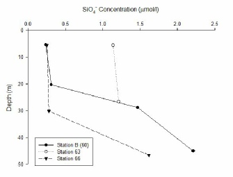
Silicon concentration increases with depth at all station with low levels of silicon in the surface waters. For station B silicon concentration is low from 0-20m, for station 66 concentrations are low from 0-30m. Below these depths silicon concentration rises to a maximum; 1.62 µmol/l for station 66 and 2.21 µmol/l for station B. Due to the presence of a strong seasonal, pycnocline mixing of nutrients into the surface layers from the deep is limited. This coupled with the removal of silicon from phytoplankton explains why there is a low concentration in the surface and higher silicon concentrations in deeper waters. As the stations move away from the coast (station 63 closest, station 66 furthest away) silicon concentrations decrease. For example station 66 has a concentration of 0.25 µmol/l (5m) compared to station 63 with a concentration of 1.14 µmol/l. This is a result of the distance of the stations from riverine input which provides a high input of silicon.
FIGURE 18; line graph showing the changes in silicon concentration with depth
FIGURES 6-12; graphs to show temperature and salinity depth profiles of the stations sampled offshore. Figure 6 (top left) shows the aforementioned profiles for station 60, figure 7(top middle) shows station 61, figure 8 (top right) shows station 62, figure 9 (middle left) shows station 63, figure 10 (middle centre) shows station 64, figure 11 (middle right) shows station 65 and figure 12 (middle bottom) shows station 66.