Group 8 - Falmouth 2015
Estuary
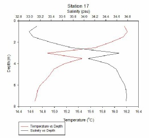
Temperature and salinity were measured using the CTD that was attached to the the rossette. The graphs below show the temperature and salinity profiles for all the stations sampled by group eight and group four.
Throughout the estuary temperature decreases with depth and salinity increases with depth. In general temperature in the upper estuary is greater than that closer to the estuary mouth, with exception of stations 26 and 27. River water entering the estuary is warmer than sea water, and flows above due to density differences. Salinity is lowest at depth in the upper estuary, and most saline water is seen at the surface near the estuary mouth; since denser, more saline sea water sinks below fresher river water. All graphs show salinity spikes, which are caused by lag from the CTD sensor.
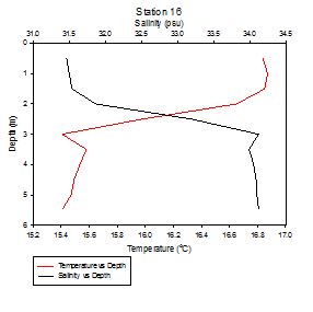
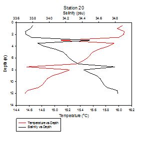
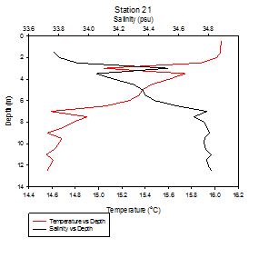
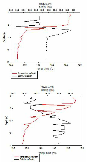
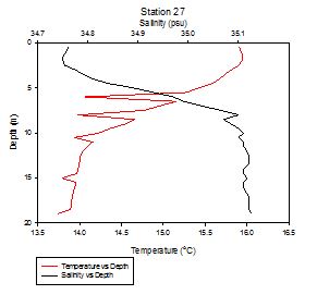
FIGURES 4-10; line graphs showing the change in temperature and salinity with depth for all the stations sampled by groups 8 and 4. Group 4 stations are
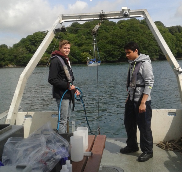
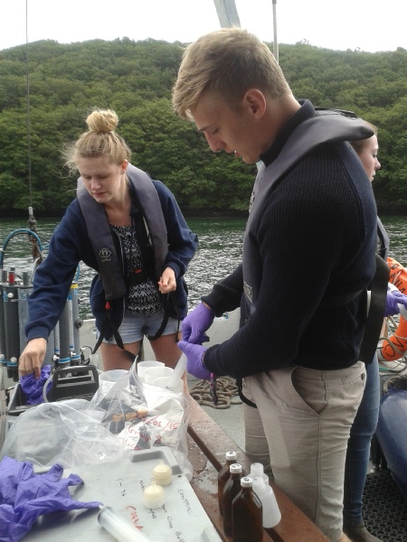
The upper Fal estuary was navigated via a small research vessel, the Bill Conway, on the morning of the 25th of June 2015. Observations were then continued on the lower Fal estuary by Group 4 in the afternoon. Sampling locations were predetermined and measurements were then obtained using a combination of automatic and manual methods. A rossette containing a CTD and 3 Niskin bottles was deployed at each station. Niskin bottles were used to collect water at different depths for manual analysis of at a later date. The CTD allowed for the obtainment of various measurements; chlorophyll, temperature, salinity, dissolved oxygen and turbidity. A plankton net was also used to collect zooplankton at one station by group eight and two stations by group four for identification, and samples were taken at every station from Niskin bottles and preserved with iodine ** for phytoplanktoun identification. An ADCP was used to measure the current speed at all depths in the river.
Disclaimer; the views and opinions expressed are those of the individual and not necessarily those of the University. ©El Sharkke 2015
FIGURE 1 (left); Richard and Hattan deploying the CTD.
FIGURE 2 (right); Kris and
Katherine doing chemical analysis.
FIGURE 3; Map of Fal Estuary showing the stations sampled by group 8 and group 4 on the 25th June.
ADCP
The Richardson Number was calculated using salinity, temperature and depth from the CTD data to calculate density and the ADCP data to give current velocity with depth. The Richardson Number gives an indication of the type of flow and the subsequent mixing as a result. If Ri is >1 flow is laminar, <0.25 flow is turbulent, and 0.25-1 it is transitional between the two types of flow.
Flow remains laminar with depth across most stations, although Richardson Number tends to decrease with depth as a result of bottom waters interacting with the sediment floor. All stations transition from laminar to turbulent flow at lower depths, such as station 17 which transitions below 5m with turbulent mixing occurring below 6m. Along the estuary (station 16 – station 21) there is little variation in this general trend of the Richardson Number with depth.
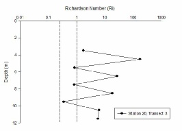
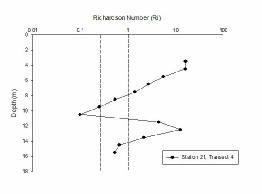
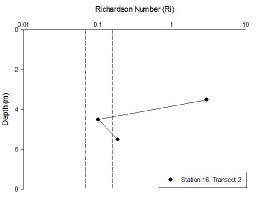
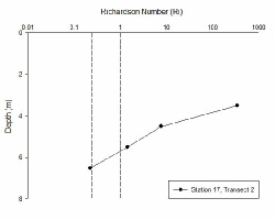
FIGURES 19, 20, 21 and 22; line graph showing the Richardson Number with depth at stations 16, 17, 20, and 24. The vertical lines represent laminar flow at >1 Ri and turbulent flow <0.25.
FIGURE 15 (left) and FIGURE 16 (right); as above for figure 11 and 12
FIGURE 17 and FIGURE 18; as above with figure 11 and 12
The rosette deployed had attached to it () Niskin bottles. From the niskin bottles we collected samples that were then used to obtain data concerning the stratification of chlorophyll present within the water column at 3 different depths, including lower, intermediate and surface. The specifics of these were adapted to the total depth of the water column which was determined via the instruments located on the research vessel. Samples were also taken and retained on glass fibre filtering paper, preserved in acetone and then analysed at a later date in the lab.
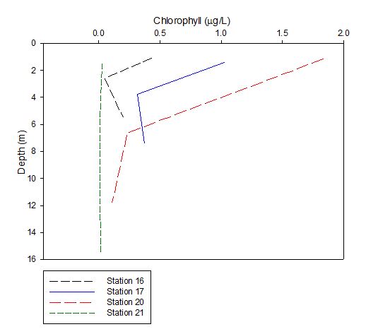
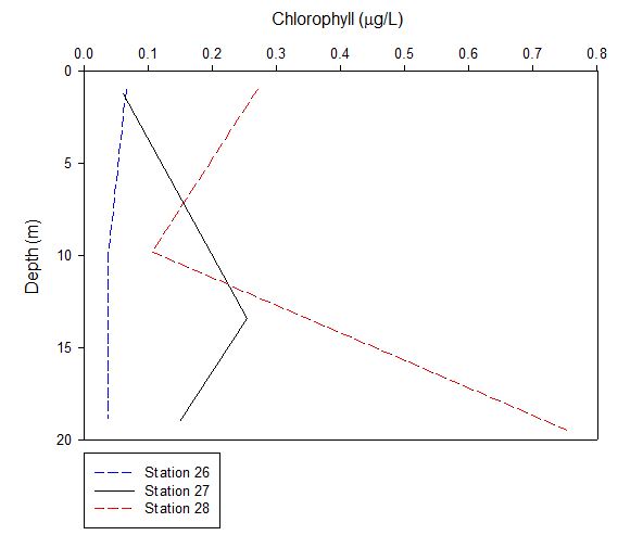
FIGURE 23 (left) and FIGURE 24 (right); line graphs showing the change in chlorophyll concentration with depth for the stations sampled by group 8 in the upper estuary (Figure 4) and group 4 in the lower estuary (Figue 5).
In general chlorophyll concentrations are much greater at the surface of the water column than at depth, with the biggest decreases between the surface and mid depth sampled. Phytoplankton prefer surface waters where light levels are highest, so are not growth limiting. Station 21 is an exception, where levels are almost constant at 0µg/L, regardless of depth. At stations 16 and 17 chlorophyll concentrations increased between the middle on the water column and depth, however not by a significant amount. This would suggest that phytoplankton growth was limited at station 21, potentially due to lack of nutrients. Highest chlorophyll concentrations, of about 1.75µg/L, were measured at station 20.
Stations 26, 27 and 28 were closer to the mouth of the Fal estuary. All three stations have very low chlorophyll concentrations, below 0.3µg/L, suggesting little phytoplankton activity. Growth here is likely to be limited by lack of biolimiting nutrients, similar to station 21. Station 26 sees a decrease in concentration with depth. Concentrations at station 27 increase slightly between the surface and mid depth, below which concentration decreases. Between the surface and mid depth, at station 28, chlorophyll concentration decreases, however the bottom sample at station 28 is an exception with a concentration of 0.75µg/L.
Zooplankton
Zooplankton was sampled at one station in the upper estuary and two stations
in the lower estuary by plankton net. The number of zooplankton per m3 of water sampled
was calculated using the number of . Zooplankton were identified under microscopes
in a Bogorov chamber that held 10ml of sample water. We have calculated the number
of zooplankton per m3
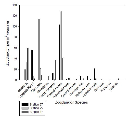
Figure 33 shows the number of zooplankton individuals per m-3 of water sampled at station 25 in the lower Fal estuary, in which the data was collected by group 4. The most abundant zooplankton species observed was decapoda larvae, at around 80 individuals per m-3, followed closely by copepod at 75 individuals per m-3. The least abundant species present were Copepod nauplii, Gastropod larvae, Chaetognatha and Tunicata jointly, occurring at densities of 4 individuals per m-3 of water sampled.
Station 27, which was also in the lower Fal estuary measured by group 4 on the 2X/6/15
at XX.XXpm UTC/BST. At this station, Cladocera was by far the most abundant zooplankton
species found, occurring at densities of 115 individuals per m-3, followed by Cirripedia
at 58 individuals per m-3. Copepod nauplii much more abundant at this station than
they were at station 25, with densities of 55 individuals per m-3 occuring. Gastropod
larvae was the least abundant species present in this sampling area at just 1 individual
per m-3 of water sampled.
Station 17
FIGURE 33; Bar chart showing the composition of the zooplankton community at stations 17, 25 and 27.
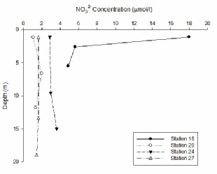
At station 16, the top of the Fal estuary, nitrate concentration decreases significantly with depth. At the surface the concentration is extremely high, at 18.0μmol/l, levels then decrease to around 5.0μmol/l at depth. At stations 20, 24, 27, further towards the mouth of the estuary, nitrate concentration is fairly homogeneous regardless of depth. One possibility for the difference in profiles is that nitrate in the surface waters of the upper estuary was used up by phytoplankton before it could be transported down the Fal.
Nitrate TDL
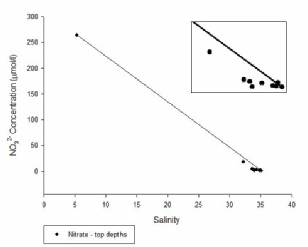
The estuarine mixing diagram shows a non conservative trend, with nitrate being removed from surface waters in the Fal estuary. It is not possible to draw any conclusions about the actual cause of removal, however one hypothesis could be removal by phytoplankton.
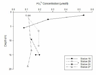
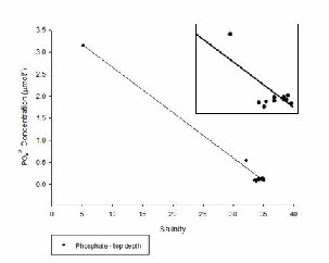
In the Fal estuary, phosphate follows similar trends to nitrate. Phosphate concentrations at station 16 decrease with depth, from just over 0.5μmol/l to less than 0.1μmol/l. At the other 3 stations, 20, 24 and 27, phosphate concentrations are fairly constant down the water column, varying between 0.1μmol/l and 0.2μmol/l, similar to the nitrate profiles at these stations. Phosphate could potentially be removed by phytoplankton in the estuary.
Phosphate TDL
The estuarine mixing diagram shows removal of phosphate further up the estuary. At the bottom of the Fal estuary, phosphate begins to show a conservative pattern. One station at the top of the estuary, with a salinity of around 32 and concentration 0.5μmol/l, suggests addition of phosphate, although more stations would need to be sampled to determine whether or not this was an outlier.
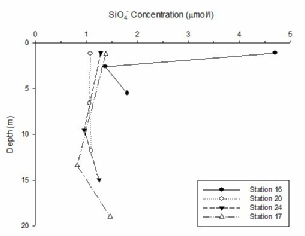
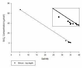
Silicon is found in very high concentrations in surface waters at station 16, 4.7μmol/l, and decreases by around 3.0μmol/l, with depth to the bottom of the estuary. Station 20, has a homogeneous dissolved silicon profile, of just over 1.0μmol/l, at all depths. Stations 24 and 27 have similar concentrations of dissolved silicon at the surface of the Fal estuary and at depth. At mid-depths both stations see a decline in concentration. This could potentially caused by the subsurface chlorophyll maxima, but would need further research to prove this theory. At all stations the concentration of dissolved silicon greater at the bottom of the estuary than at mid depths. This could be because dissolution of diatom frustules at depth, although again this cannot be concluded for certain.
Silicon TDL
The mixing diagram shows slight removal of dissolved silicon in the upper estuary and conservative mixing near to the mouth of the Fal. This suggests that diatoms, which require silicon to form their frustules, are abundant in the upper estuary, but not present in significant numbers in the lower estuary. This is just one possible reason for removal and cannot be concluded without further evidence.
FIGURE 30; shows the change in silicon concentration with depth for stations 16,
20, 24 and 27.
FIGURE 31; estuarine mixing diagram for silicate.
Nutrients
FIGURE 26; shows the change in nitrate concentration with depth for stations 16,
20, 24 and 27.
FIGURE 27; estuarine mixing diagram for nitrate
FIGURE 28; shows the change in phosphate concentration with depth for stations 16,
20, 24 and 27.
FIGURE 29; estuarine mixing diagram for phosphate
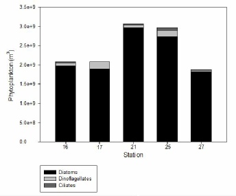
We can see from Figure 32 that Diatoms are the dominant phytoplankton genera, forming the large majority of the phytoplankton biomass, followed by Dinoflagellates and then by Ciliates, as is observed across all of the stations. Stations 16-27 extend down the estuary towards the seaward end. The largest phytoplankton biomass is seen at station 21 which is mid estuary where conditions may be optimum for growth due to the balance of nutrient input from the riverine end and higher salinities of the seaward end. No Ciliates were found at Station 17. There are many other interlinked factors affecting the variations in growth such as turbidity, light attenuation, dissolved oxygen concentration and water temperature which vary over the length of the estuary due to the mixing between the river and the sea.
Samples of water were collected using niskin bottles attached to the rossette. Samples were preserved in **dide. In labs we then identified and counted under a microscope the phytoplankton cells. We calculated the number of phytoplankton cells per m3 and below is a graph showing our findings.
Dissolved oxygen
Water samples were taken from the estuary and later analysed in the lab to find the dissolved oxygen concentration. The graph below shows the results from the surface water samples from group 8 and group 4’s sites on the estuary.
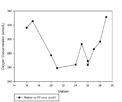
This graph shows the changes in the O2 concentration levels down the estuary in the surface waters. Station 14 was taken at the furthest point upstream that Conway could reach which is, for the record, a long way from the rivers end point. There are obvious differences down the estuary. At either end there are points of maximum concentration. In the middle of the estuary there are very low levels of dissolved oxygen recorded. In figure 4 station 21 shows extremely low chlorophyll levels. This indicates that there is very little primary productivity and therefore there will be a net loss of oxygen as a variety of other organisms living there use it to respire. This leads to the low levels of dissolved oxygen seen at this point in this figure.
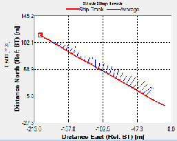
FIGURE 11 (left); shows the ship track with current direction
FIGURE 12 (right); shows
the current speed at different points in the river
FIGURE 13 (left) and FIGURE 14 (right); as above for figure 11 and 12
FIGURE 25; line graph showing the change in dissolved oxygen in the surface waters for all the stations sampled by group 8 and group 4. Station 16 is the least saline water (upper estuary) and station 29 is the most saline water (lower estuary).
Flow velocities on the west of the estuary are greater, with maximum velocity of 0.388ms-1. Velocities in the centre of the water column and in the east are lowest, below 0.200ms-1. At the top of the estuary flow speeds greatest measured in the estuary overall. …(maybe related to tides)…

Maximum velocities are seen at the top of the water column, on average around 0.195ms-1. The predominant flow direction is north/north east into the estuary.
FIGURE 32; bar chart showing the composition of the phytoplankton communities for the surface water samples taken for stations 16-27. Station 16 is the uppermost station of the estuary and station 27 is the lowest station of the estuary.
On the centre and east of the estuary, water is moving north into the estuary, at flow velocities of around 0.200ms-1. However on the far west water is moving out of the estuary rapidly at 0.250ms-1 to 0.255ms-1.
In the centre of the estuary flow velocities are greatest (0.150ms-1), with flow predominantly moving northward in the estuary. Additionally, there is another area of increased velocity (0.088ms-1) along the seabed on the west. This is moving south, out to sea. At this station flow velocities were slowest.