Estuary

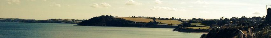
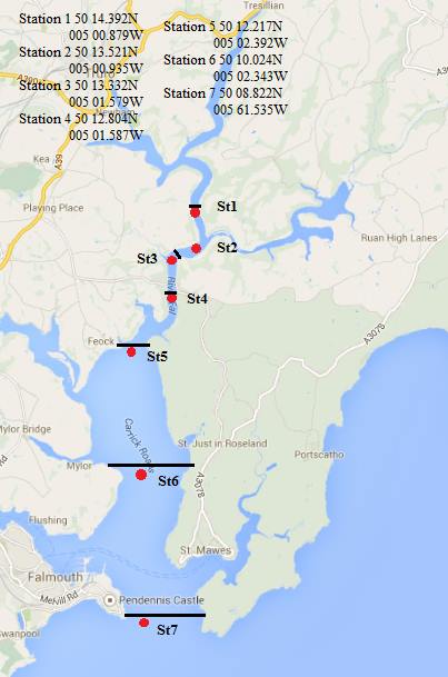
Our group went out into the Fal Estuary on the 25th June 2014 on the Bill Conway and collected data from 7 sites in the estuary between Woodbury Point (50.14.392 N, 005.00.879 W) and Blackrock (50.08.822 N, 005.61.535 W) which are shown on the map below. The sites selected were chosen to represent the whole of the estuary and included sites which may have had significant characteristics; including fish farm and the confluence of the Fal and Truro Rivers into the estuary. As it was low tide when sampling began, it was important to start at the top of the estuary to ensure the same body of water wasn’t sampled as it moved down the estuary. On the day of data collection high tide was at 0435 UTC and low tide was at 1116 UTC and weather conditions were calm, but overcast.

The data that we collected from the estuary included;

• ADCP transect
• CTD depth profiles
• Various nutrient concentrations using water samples from multiple depths
• Zooplankton and phytoplankton sample

Biology

At three sites in the estuary we used a 200 micron zooplankton net to collect a 1 litre water sample to be used to estimate the species and number of zooplankton at different points in the estuary. The zooplankton net was cast at sites 1, 5 and 7. We also collected a separate water sample at the first site which was used to estimate the species and number of phytoplankton in the estuary.

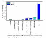
Phytoplankton: The most abundant phytoplankton observed was genus Chaetoceras (Figure 1), which is expected as Chaetoceras is the largest genus of phytoplankton (Atlas, 1984), and can be present in regions with vast environmental ranges, from oceanic temperatures of below freezing to thirty degrees Celsius, and salinity gradients from eighteen in estuarine systems, to over thirty five.  Thalassiosira rotula was the second most abundant phytoplankton observed.  

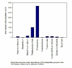
Zooplankton: The most abundant zooplankton samples observed were copepods, which is to be expected, as well as decapoda and cirripedia larvae (Figure 2).

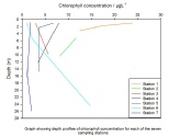
Chlorophyll: At each site chlorophyll concentrations varied with depth (Figure 3). Sites 1, 2, 4 and 5 showed an overall decrease in chlorophyll concentrations with depth with changes of 10.4µgL-1, 3.45 µgL-1, 4.51 µgL-1 and 3 µgL-1 respectively. Site 1, 2 and 4 showed relatively consistent decreases with depth whereas site 5 indicated a rapid decrease in the first two meters and then the rate of decrease slowed. Sites 3 and 6 showed an increase in chlorophyll concentrations with depth. Site 7 showed a decrease in chlorophyll concentration in the first 16 meters but then the chlorophyll concentration starts to increase and reaches a level similar to the surface concentration. Figure 4 shows the relationship between percentage oxygen concentration and chlorophyll concentration. Higher values of chlorophyll are associated with higher oxygen saturation levels, however there is some scatter around the line of best fit.  

Chemistry

At each site water samples were collected from different depths which were used to determine the concentrations of dissolved oxygen, chlorophyll, silicon, phosphate and nitrate. The nutrient data shows how the concentrations of different nutrients vary along the depth profile of the water column.

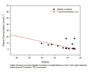
Silicon: Silicon concentrations show that dissolved silicon is a conservative nutrient in the Fal estuary. The concentrations are higher in the lower salinity regions higher up the estuary and decrease with increasing salinity. The river end member which had a salinity of 7.3 had a dissolved silicon concentration of 63.6461 μmolL-1 whereas the saline water end member which had a salinity of 35.204 had a dissolved silicon concentration of 0.4478μmolL-1. (Figure 1).

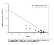
Nitrate: The estuary mixing diagram for nitrate indicates negative non-conservative behaviour, but it should be noted that there is little data for low salinities other than the river end members. At the river end member the salinity is 7.3 and the nitrate concentration is 444.8289, at the saline water end member the salinity is 35.005 μmolL-1 and the nitrate concentration is 0.4943 μmolL-1. The data shows that nitrate concentrations decrease with increasing salinity but that at higher salinities there is more fluctuations in the concentration of dissolved nitrate. (Figure 2).

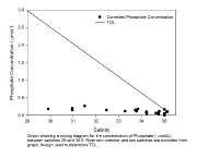
Phosphate: Phosphate concentrations remained consistently low across all sites in the estuary except at the end members highlighting non-conservative behaviour. The measurements of phosphate concentrations were all around 0.1-0.2 µmolL-1 at each site across the estuary. Mixing diagrams show consistently high salinities, even at the top station within the estuary, it should be noted that data was collected after a period of very minimal rainfall. (Figure 3).

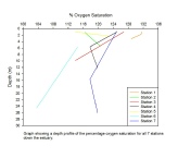
Dissolved Oxygen: The dissolved oxygen concentration decreased with depth at sites 1, 3, 4, 6 and 7. Each of these sites showed a varied rate of decrease in dissolved oxygen with depth. At sites 2 and 5 the concentration of dissolved oxygen increased with depth. (Figure 4).

Physics

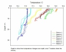
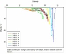
CTD: At each site a CTD was used to create depth profiles to show changes in the water column along the estuary. The major changes in the depth profile showed that temperature decreased with depth and salinity increased with depth. The CTD profiles indicated that temperature was highest at the top of the estuary and decreased with distance downstream (Figure 1). The salinity profile showed that the lowest salinity is at the top of the estuary and increased with distance downstream. The salinity profiles also showed that the salinity profile became more uniform at sites 5-7 further downstream. This indicates that the Fal is a partially mixed estuary (Figure 2). The transmission also changed along the estuary showing that the transmission increased with increasing distance downstream. At the sites 1-5 there was a slight increase in transmission with depth whereas sites 6 and 7 showed a fairly uniform turbidity profile. Fluorescence is most variable at the top of the estuary, as was the highest value, which was measured at 3.4m depth as 1.5 volts at station 1. Towards the bottom of the estuary fluorescence is much lower and less variable with depth.

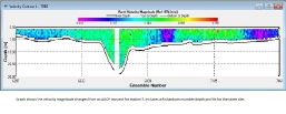
ADCP: At each station ADCP data was used to show how flow velocities changed with both distance across the estuary and depth (Figure 3). At station 1 in the upper estuary, the flows were highly variable with no obvious changes with depth or position. Moving further south, stations 2, 3 and 4 showed fairly uniform flow velocities of 0.2 to 0.5 m/s across the estuary. As the transect distances increased as width of the estuary increased towards the mouth, more variation in flow speed was observed, with station six showing a maximum speed in the deepest part of the channel. Station 7 (Figure 4) showed great variation in flow speeds, generally being higher in the deep channel than in the shallower areas to either side.

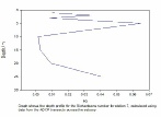
Richardson’s Number: Using the data from the ADCP and CTD we were able to calculate the Richardson’s number (Ri) for the water column and compare the degree of mixing at the different study sites. At site one we found that the Ri values showed that mixing was likely at the top of the water column and that mixing was unlikely at the bottom of the water column. This would be expected because there was a larger difference in density in the last metre of the water column compared to the first half metre. The other study sites showed varying but consistently low Ri values throughout the water column indicating that mixing is likely with the exception of site 6. Site six was located at the confluence of the Fal and Truro Rivers which meant that there was an additional input of freshwater which implies that the water column would have been stratified. The Ri value for the first 5 metres of the water column suggests that mixing is likely, which is expected because the freshwater is itself mixed due to the low variation in density. The middle of the water column had a Ri value indicating that mixing was unlikely which can be explained by the relatively large differences in density and the large spatial scale that was used for the Ri calculations at this site. The bottom of the water column at site six showed that there was a transition stage at approximately 15-20m and below that between 20m and 25m mixing was likely. Depth profiles were then generated from this data for each site (Figure 4).

Discussion

Chaetoceras and Thalassiosira rotula were the most common genus groups observed in our samples.  This was to be expected as they are thought to be the most abundant genus’ of phytoplankton[1].  These cells were observed in the lab; they were discoid, and connected in an observable chain by ciliates.  Under observation we were able to observe cell chloroplasts surrounding the cellular walls.  

Copepoda was the most abundant zooplankton group observed, which is also expected as they dominate zooplankton populations in most regions[2].  It is however worth nothing that in high abundances, Thalassiosira rotula have potential to create higher than usual polyunsaturated aldehydes which can be harmful to copepod population stability[3]; Falmouth Estuary is tidal dominated and because of this there is not as much nutrient influx to create an over abundance of these phytoplankton groups, meaning that diversity remains wide in the system.

At station 1 the water column was well mixed as a result of the tidal dominated system in the Falmouth Estuary.  We sampled station 1 first and did so during the high water, working against the incoming tide as we proceeded outwards towards the sea.  

At station 2 we observed the lowest salinity values, despite being further down the estuary, due to the convergence of two fresh water bodies inputting into the estuary.  Between stations 2 and 3 the salinity profiles turned to that of a salt wedge system, which demonstrated partially mixed behaviour.  However, the salt wedge profile quickly dissipated towards station 3 as a result of the sedimentation at the mouth of the rivers inhibiting freshwater flow in great velocity.  At station 3 the system again became partially - well mixed with multiple [two] partially mixed layers.   

Turbidity was highest at stations 2 and 3 at the confluence of the River Fal and the Truro River; these effects became less influential as we approached the opening to the estuary at Carrick Roads.   

Stations 3-5, located in the Carrick Roads region of the estuary showed non-conservative nutrient behaviour; flocculation of nutrients decreased where turbidity declined.  

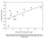
Chlorophyll concentrations were observed highest at station 7, furthest down the estuary towards the sea.  The transmission of available light increases in regions with less turbidity and reduced particulate matter and flocculation occurring; there was less of a scattering effect the further down the estuary we went.  Due to the estuarine systemic well-mixed properties, the deeper penetrating light in the open estuary resulted in increased distribution of nutrients throughout the water column.  

Figures 1-4 for nutrients show non-conservative behaviour in phosphate and nitrates, and conservative behaviour in silicates.  Due to the fact that our survey was conducted in the summer months, after major phytoplankton blooms have occurred, the behaviour of dissolved silicates would be expected to be conservative.  

[1]Bergkvist, J. (2012). Grazer-induced responses in marine phytoplankton.

[2]Lauria, M., Purdie, D. and Sharples, J. (1999). Contrasting phytoplankton distributions controlled by tidal turbulence in an estuary. Journal of Marine Systems, 21(1), pp.189--197.

[3]HERN\'ANDEZ-BECERRIL, D. (1993). Note on the morphology of two planktonic diatoms: Chaetoceros bacteriastroides and C. seychellarus, with comments on their taxonomy and distribution.Botanical journal of the Linnean Society, 111(2), pp.117--128.