Falmouth - Group 5

Disclaimer: The views expressed within this website do not represent the views of the National Oceanographic Centre of Southampton; University of Southampton; or Falmouth Marine School. We would like to thank Falmouth Marine School for the collaborative efforts involved.

Home Offshore Estuarine Geophysical Pontoon

CTD

Biological

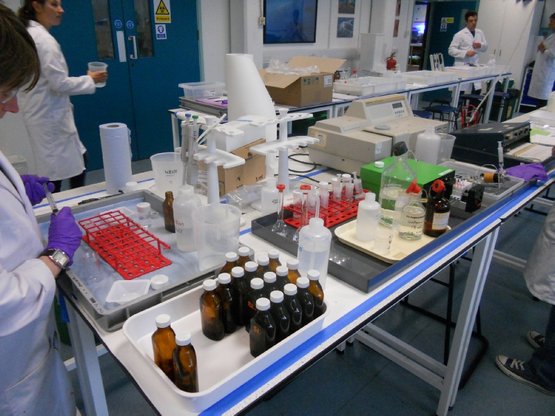
Phytoplankton Lab

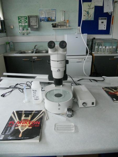
100ml of phytoplankton samples were preserved with formalin and stained with in Lugol’s Iodine. 90ml of excess Lugol’s iodine was removed and 1ml of the sample was analysed in a Sedgewick-rafter chamber under a microscope and phytoplankton cells counted over 5 transects of 20 squares. As the sample was concentrated by a factor of 10x the values were multiplied by 10 to represent the number of cells per ml.

Zooplankton Lab

The trawl samples had been preserved in formalin over night. The following morning the contents of each sample were estimated using a Bogorov Chamber. The list below contains some of the more common zooplankton groups found in the samples:

Phytoplankton

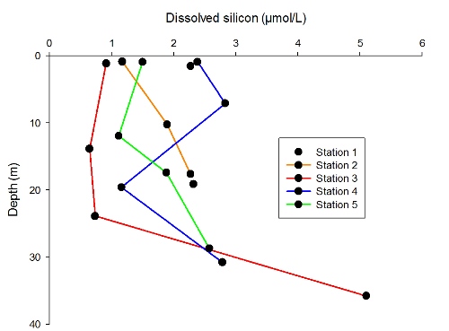
The diatoms Chaetoceros, Pseudonitzchia and Coscinodiscus were fairly ubiquitous at Station 1. The dissolved silicon profile at this station was relatively uniform with depth, suggesting that these diatoms were evenly distributed through the water column.

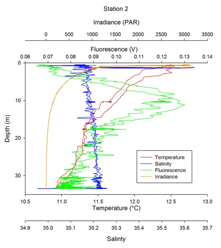
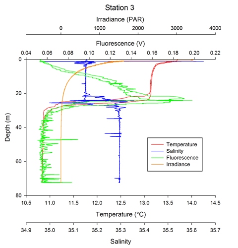
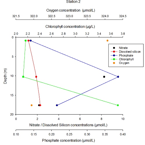
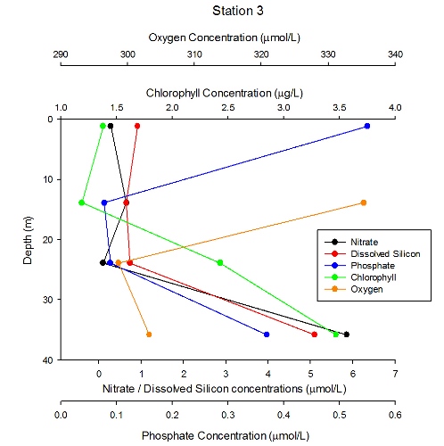
At station 2, the dissolved silicon profile exhibits a decrease to ~12m, and an increase below this depth (figure). Table shows that the diatom species found at this station are largely limited to the upper layers of the water column, generally being found in their highest abundances above 17m. Similarly, at station 3, most of the diatom species are found in the upper 23m of the water column. Dissolved silicon concentrations are relatively uniform above this depth, and concentrations increase below, see salinity.

Leptocylindrus danicus and Thallasiosira spp., diatoms often associated with deep chlorophyll maxima (DCM) (Kemp et al, 2000), were found between 17m-20m, see Table. Although Rhizosolenids are also a genera typical of DCM (Kemp et al, 2000), they were generally found in these samples in shallower water than the Thallasiosira spp. They do appear at ~20m at station 4 however, where there is evidence for a DCM. The dissolved silicon profile for station 4 supports the idea of a DCM, as concentrations decrease sharply from ~10m to ~20m, indicating the presence of diatoms between these depths.

The dinoflagellates Alexandrium and Karenia mikimotoi were associated with station 5, close to the front, see Table. This is perhaps to be expected, as dinoflagellates are often found at frontal systems.

Zooplankton

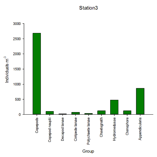
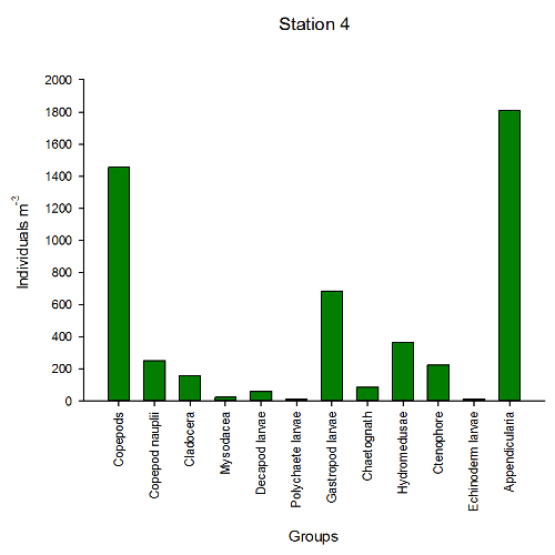
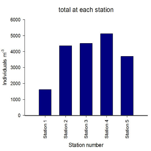
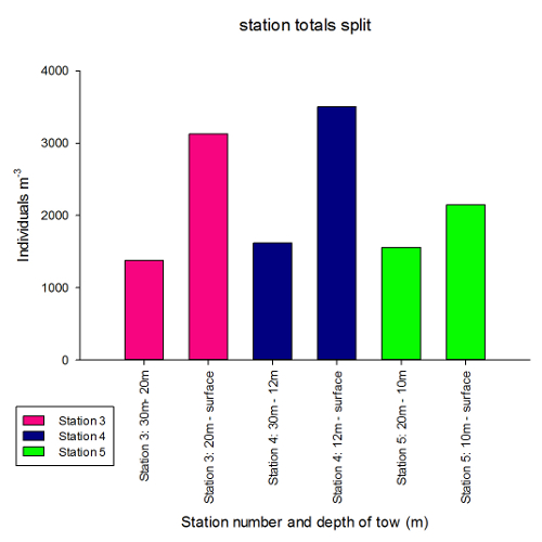
The highest number of individuals per m3 was found at station 4, as seen in (fig.), which also has a wide band of backscatter visible on the corresponding ADCP data. Station 3 has two bands of backscatter visible in ADCP, one at ~20m and another, slightly narrower band at ~10m. Station 3 had a high total abundance of zooplankton, with the highest numbers being found in the 20m – surface tow, which would have passed through both these layers.

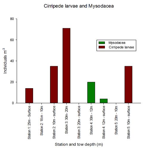
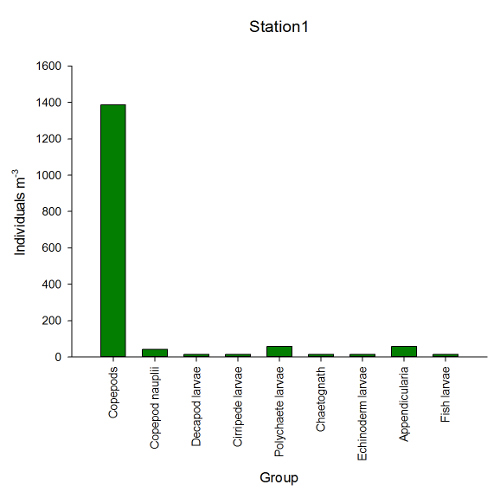
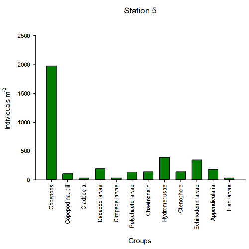
Cirripede larvae were not found at station 4, and were found in their highest numbers at station 3 between 20m -30m. Given that barnacles are a coastal species, it is perhaps to be expected that larvae would not be found at the station farthest offshore. Mysodacea (water fleas) were only found at station 4, see graph to the right.

As expected, copepods dominated at all stations except station 4. Copepod dominance was particularly notable at Station 1, where they accounted for 86% of the total sample. This dominance of copepods is consistent with results from other North Atlantic coastal stations, including station L4 off Plymouth, where copepods often account for between 60%-90% of samples (Eloire et al, 2010).

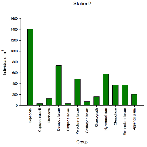
The diversity of each station is difficult to estimate due to the fact that copepods were not identified to species level. However, station 2 had the most “even” profile, with the highest abundances of echinoderm, polychaete and decapod larvae. Although copepods were the dominant group found here, it was a less pronounced dominance than at other stations, accounting as they did for only 32% of the total sample, see graphs to the right.

Appendicularians were also prevalent in samples from stations 3 and 4, indeed, they were the dominant group at station 4. High abundances of appendicularians have been noted in previous studies of the zooplankton of the Western Channel in the summer (Eloire et al, 2010), so it is likely that our results are indicative of the seasonal pattern of the area.

Vertical tows were performed with a 200µm net so it is possible that some of the smaller zooplankton species may not have been sampled.

Chemical

Chlorophyll

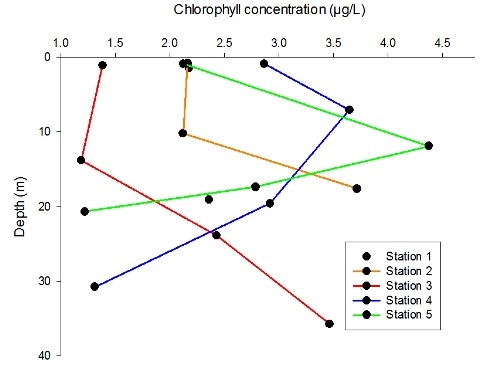
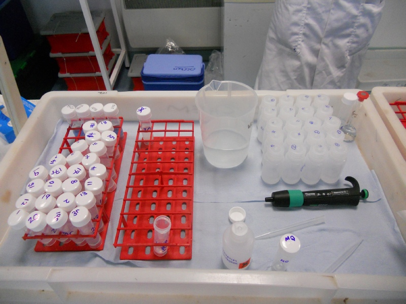
For each Niskin water sample, two chlorophyll samples were collected on 0.7µm glass fibre filters. The filters were stored overnight in acetone and measured as per the protocol stated by Parsons et al (1984). Similar to the Fluorometry data, Deep Chlorophyll Maxima were discovered at depths that varied between each station, and not much was found at Station 1.

Nutrients

Sub-samples were taken from each Niskin bottle for the measurement of phosphate, nitrate and dissolved silicon. Two samples were taken per bottle, one just for silicon and one for both nitrate and phosphate. The samples were 50 millilitres of seawater pressure filtered into labelled bottles to remove organisms and aggregates. The dissolved silicon analysis required storage in plastic bottles while the phosphate and nitrate sample was stored overnight in a glass bottle.

Phosphate and dissolved silicon levels were measured as per the protocol stated by Parsons et al (1984) using a U-1800 spectrophotometer. The calibration for the machine has been provided by Falmouth Group 6, and we would like to thank them for this data. Silicon absorption wavelength was set to 810nm and phosphate to 882nm.

Nitrate was measured using flow injection analysis as per the protocol stated in Johnson and Petty (1983).

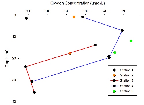
Oxygen

Dissolved oxygen was measured as per the protocol stated in Grasshoff et al (1999). The data for some stations is sporadic as some data points are missing. The equipment malfunctioned and backup phials were not taken; great care should be taken in the mixing process during titration.

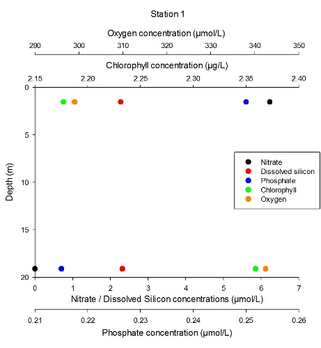
Station 1

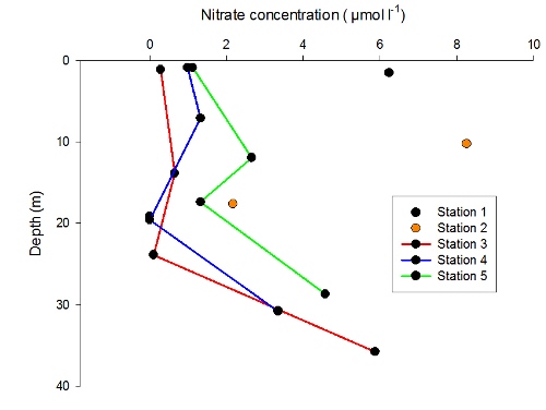
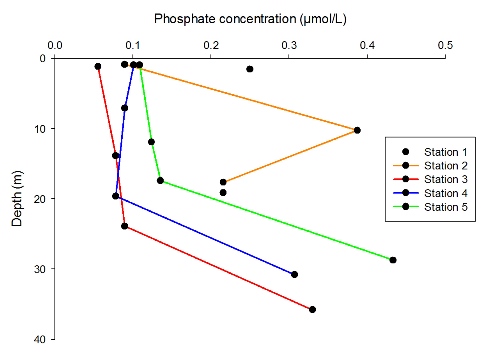
There is a relatively deep chlorophyll maximum at depths recorded slightly higher than a similar structure at Station 2. Dissolved silicon is relatively constant throughout the water column. Phosphate is present in slightly higher concentrations at the surface than at depths and nitrate is much higher in surface waters than at depths, see graph to right. This is due to the riverine inputs at this station as it is located at the mouth of the Fal Estuary at Black Rock. The results from the nutrient profiles suggests substantial mixing due to tidal impacts or freshwater inputs. However, nitrate seems to be absent from deeper waters, which contradicts mixing theory, however it may be depleted by phytoplankton.

Station 2

Due to the location of Station 2, a DCM should be noticeable. However, instead there is a low chlorophyll value seen at 10m depth, equating to 2.12ug.L-1. The highest chlorophyll levels are seen at 17.6m depth, 3.72 ug.L-1. This may be a result of phytoplankton residing in deeper waters at this time of day rather than migrating to the surface. Variances in nitrate and phosphate concentrations within the water column suggest that there is significant primary production at this site and phytoplankton move to deep waters to obtain nutrients. It seems this region has some stratification. Dissolved silicon concentrations are relatively uniform throughout, see graphs to the right, which suggests that there are little (if any) populations of diatoms in this region, find out here.

Station 3

Station 3 shows a chlorophyll maximum of 3.47 ug/l at 35m depth. Nutrients show significant change throughout the water column, with nutrient concentrations being high in deeper waters, although phosphate was found to be very high at the surface. It would seem that, like station 2, there is stratification and migration of phytoplankton. However, unlike station 2, there were variations in dissolved silicon concentrations with depth, see graph to the right, suggesting that perhaps diatoms are present even though waters may be stratified, see biology.

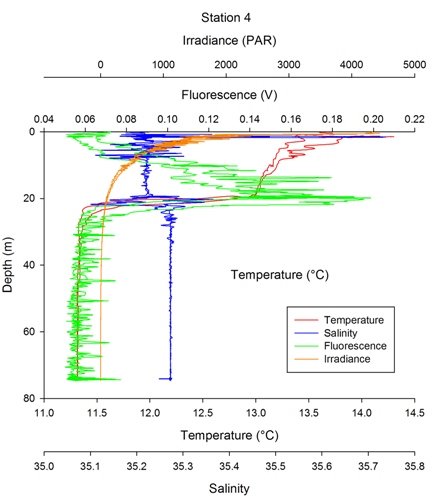
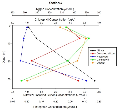
Station 4

Dissolved oxygen and chlorophyll have similar vertical profiles at Station 4, reinforcing the assumption that chlorophyll is used as a proxy for primary production. The chlorophyll maximum, with the highest value of 3.65ug.L-1, is relatively near the surface, at a depth of 7m. This is approximately at the same depth as the maximum value of dissolved oxygen, 349.35umol.L-1. There are high dissolved silicon concentrations at this chlorophyll maximum, yet low dissolved nitrogen and phosphate. This suggests that the likely groups of phytoplankton species includes dinoflagellates, which vertically migrate to obtain an optimum of both nutrients and light; this explains their proximity to the surface during day time. Siliceous populations of phytoplankton are unexpected in this area because of the high silicon values; Silicon would be utilized in their metabolism. The low silicon values in the thermocline may suggest localized diatom populations within the gradation: the differences in temperature may induce some mixing via vertical convection.

Station 5

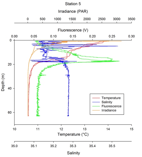
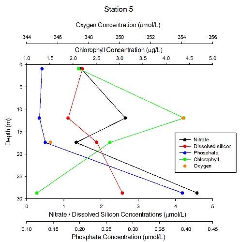
There is a chlorophyll maximum of 4.38ug.L-1 at a depth of 12m at Station 5; this is the highest chlorophyll level observed during the offshore study, see Chlorophyll to the right. The concentration of dissolved silicon is very low at the Deep Chlorophyll Maximum (DCM), see Silicon, which suggests that diatoms are present. Phosphate is also low at the chlorophyll maximum, refer to Station 5 graph, but since nitrate levels are comparably high this suggests that nitrate is not a limiting factor for phytoplankton growth near the front. Despite the fact that there are only two dissolved oxygen values, the Station 5 graph suggests that the concentration of O2 was relatively high, with a maximum value of 354.1umol.L-1 at the chlorophyll maximum, also reinforcing that chlorophyll can be used as a proxy for phytoplankton growth. As Station 5 is located close to a front, there will be some mixing, however the level of nutrients decreased rapidly below the thermocline, showing that there is still some stratification. Overall the nutrient, chlorophyll and oxygen profiles at station 5 suggest that primary production is very high at frontal zones.

Physical Separate station data can be found above and to the right

Temperature

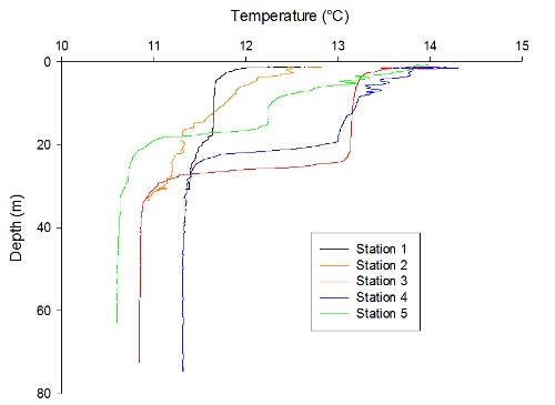
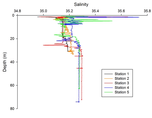
A rapid decrease in temperature, over the first few meters from the surface, was noted at all stations, see Temperature. Stations 3, 4 and 5 all had pronounced thermoclines at 25-30m, 20-25m, and 15-20m respectively. A thermocline was not evident at station 2, but rather a reasonably steady decrease in temperature with depth. Station 1 had a uniform temperature from 4.5-8.0m, after which it decreased again. The greatest variation over the thermoclines occured at station 3, with a 2.2°C temperature decrease from 13.1°C to 10.9°C, compared to 1.6°C and 1.5°C recorded at stations 4 and 5.

Salinity

Salinity remained relatively constant with depth, except for where there were haloclines present at stations 3, 4 and 5, see Salinity. At these haloclines, the salinity increased rapidly before settling out again, with variations of 0.15, 0.05 and 0.12 at stations 3, 4 and 5 respectively. At stations 1 and 2, there was a slight decrease in salinity over the whole profile. The lack of a pronounced halocline reinforces the theory of this being a more poorly stratified station. This allows a larger depth range of more optimal conditions in which phytoplankton can grow. Perhaps the greater depths of stations 3, 4 and 5 are what caused haloclines to form there, rather than at stations 1 and 2. The greatest salinity towards the surface was found at station 4, 35.22, which was the furthest away from land and freshwater influence. The opposite was true of station 1 (salinity of 35.14). The depths of the haloclines correspond to the depths of the thermoclines found in the CTD temperature profiles, suggesting a relationship between the two parameters, see graphs to the right.

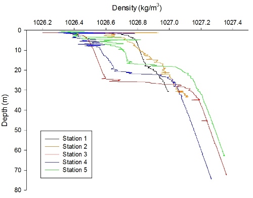
Density

All of the stations exhibit an increase in density with depth implying vertical stability within the water column, see Density. Station 1 is relatively well mixed, displaying the least variation among all stations. Such mixing patterns reflect the mixed nature of the Fal River. A steady increase of density with depth is seen at station 2 with no pronounced pycnoclines. This station was sampled at high water slack, and the absence of a pycnocline could be caused by the ebb and flow of surface waters. At stations 3, 4 and 5 the densities distinctly change at 28m, 25m and 18m deep respectively. 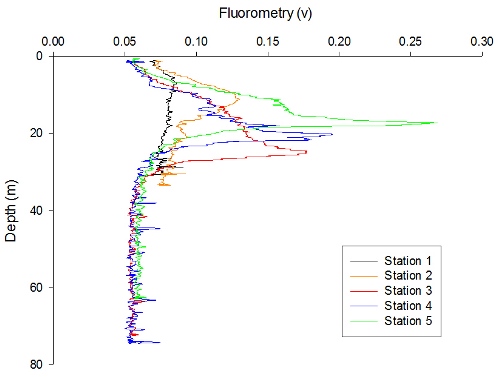Station 3 had the greatest density range of 1kg.m-3, while the least difference is held by station 1 with only 0.3kg.m-3 between surface and bottom waters. The pycnoclines that exist correspond to peaks in chlorophyll, measured (by proxy) using a fluorometer.

Fluorometry

All of the stations, except Station 1, are shown to contain deep chlorophyll maxima at varying depths, see Fluorometry. Station 2 shows a chlorophyll maximum around 10 meters depth (fluorometry reading of 0.13V); as the later stations have deeper chlorophyll maximums, this is a possible indication of vertical migration. Fluorometry spikes recorded at stations 3, 4 and 5 correspond with the pycnoclines indicated on the density graph (at ~28m, ~25m and ~18m respectively). The fluorometry spikes sit just above the corresponding pycnoclines at ~ 25m (station 3), ~20m (station 4) and ~18m (station 5), this suggests the presence of deep chlorophyll maxima at these stations. The largest spike is at station 5, which was the closest sampling point to the front.

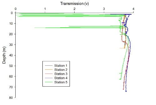
Transmission

The changes in transmission relate to the amount of Suspended Particulate Matter, SPM, in the water column; for example, transmission levels of 100v would represent clear water. On the CTD profile for station 1, the transmission ranged from 3.74v at the surface (1.23m) to 3.73v at 30.73m, as shown by Transmission; this expresses the uniform properties of the water column. At Station 2, a similar profile was seen: as depths increased, values of 3.67v at 1.17m down to 3.71v at 33.48m were recorded. At Station 3 the clarity increased temporarily, showing a possible decrease in SPM. The depth profile at Station 4 indicated an increase in SPM with depth; the transmission closest to the surface (1.22m) was 3.88v and was lower, 3.76v, at 70.50 metres. Station 5, closest to the front, showed the most variation in transmission, with the lowest recorded value of transmission (0.02v) being at 2.27m. A change in transmission however, from 0.27v to 3.55v was recorded from 0.63m to 62.91m, respectively; indicating a mass of planktonic activity near the surface, dissipating with depth.

ADCP

Backscatter intensity relates to Suspended Particulate Matter composition and size distribution (Vicente et al. 2010). There are generally low backscatter values at station 1, with minimums below 20m of 64Db as shown in figx. Both stations 1 & 2 experience random spots of high intensity backscatter within 3m of the surface; these spots are larger and more frequent at station 2. Stations 3, 4 and 5 all display uniform bands of backscatter at ~20m with varying intensities. These bands of backscatter likely allude to the presence of large zooplankton communities in the water column, with the intensity of the backscatter acting as a proxy for the population size. This would suggest that the largest zooplankton community would be found at station 4 with a very wide band of backscatter and intensity values of >80Db, see Biological for details.

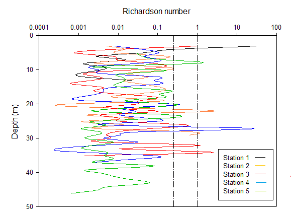
Richardson Number

There are both turbulent and laminar elements to the water column at each station, however turbulent flow is prevalent, see Richardson Number. Laminar flow is present at Richardson values of greater than one; this can be observed at ~3m depth at station 1. There are examples of laminar layers at each station; however they are primarily toward the deeper end of the profiles. There are a few plots that cross the Ri = 0.25 threshold but do not pass the Ri = 1 lag zone boundary. These would therefore be considered in a phase of transition, but would effectively remain laminar. The primarily turbulent nature of the water column encourages vertical transport of properties and the shear between the two interfaces which promotes entrainment i.e Kelvin-Helmholtz instabilities.

Stratification Index

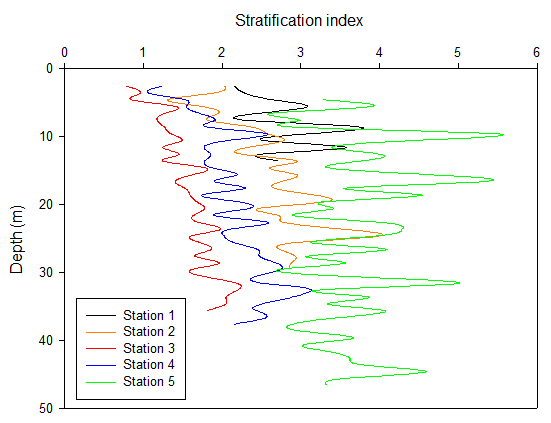
It is apparent from the Stratification Index data that Station 5 is the most stratified area of water that was sampled, with a range of values between roughly 3 and 5. This is expected at station 5 as it is the closest station to the offshore side of the front, yet is not as heavily affected by offshore influences as station 3 and 4. Station 3 and 4 are the most well mixed stations due to their distance offshore. The difference in stratification index can allude to the phytoplankton species present at each station. Larger species of phytoplankton such as diatoms would be expected at station 3 and 4, whereas dinoflagellates would be more common in heavily stratified areas. However, the presence of these communities are also nutrient dependent. For more information on the biology see the biological section.

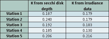
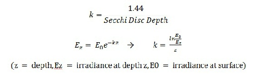
Attenuation Coefficient

The attenuation coefficient, k, was calculated for each station based on the equations below.

The two methods of calculating the attenuation coefficient, k, agree fairly well, giving similar values as seen in the above table. The attenuation coefficient is lowest at station 4, which is furthest offshore, therefore the euphotic zone is the deepest of all stations measured and has a greater depth for potential primary production.

Overview

Summary

A front was encountered between Stations 2 and 5. Station 5 produced the largest chlorophyll maximum, see here. Station 2, as expected, shows the largest measured cell count of diatoms due to its position on the estuarine side of the front, see here. Station 5 is the most stratified station with an index between 3 and 5; this corresponds to the high numbers of smaller phytoplankton species, see here. The highest number of zooplankton was found at station 3 and 4 suppressing relatively large phytoplanktonic populations. Speciation changed with distance off coast, see Biology.

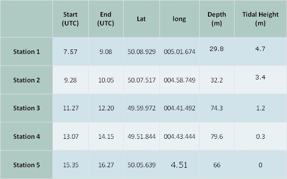
Sampling

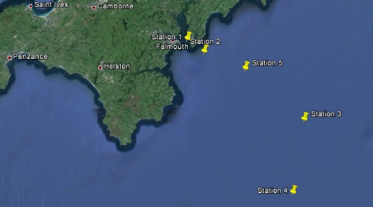
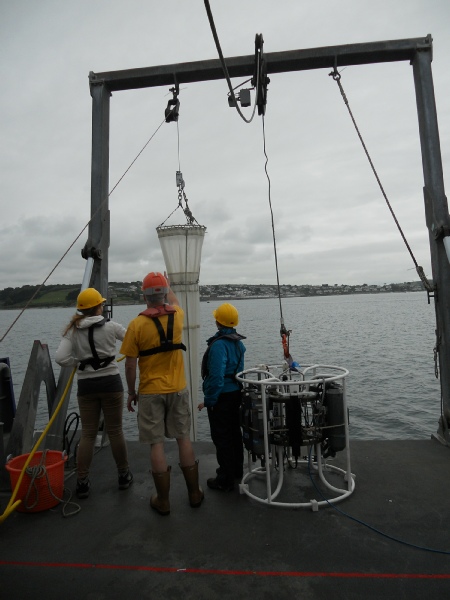
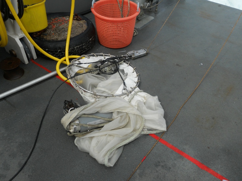
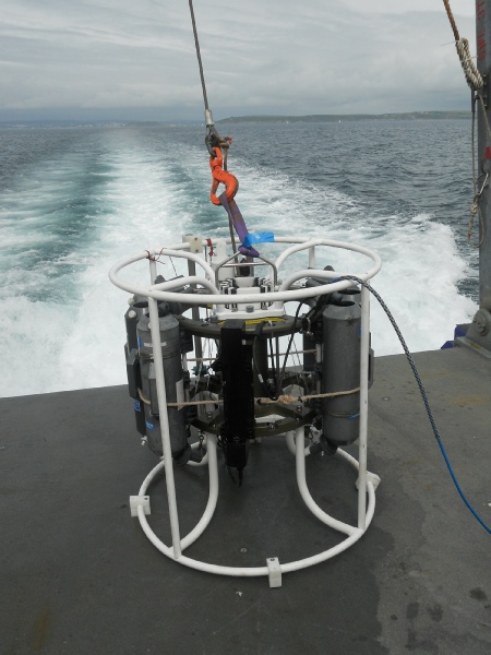
Samples were collected at 5 stations directly offshore of Falmouth in the English Channel to determine the presence and location of a front. Vertically towed nets with 200µm mesh collected samples of zooplankton at each station. Niskin bottles attached to a CTD rosette were deployed and the data from the descending CTD, found to the left, was used to determine depths to fire the Niskin bottles on the ascent. Sub-samples were taken from the Niskin bottles and then stored appropriately in order to measure chlorophyll, dissolved oxygen, silicate, nitrate, phosphate and phytoplankton at a later time. ADCP data was recorded for the duration of the boat trip. New transects were recorded for each station and for the path between each station. A Seabird Thermosalinograph recorded temperature, salinity and fluorescence whilst the boat was underway; the data from which can be seen graphically here. The front represents a transition from a nutrient depleted, warm water environment to cold water rich in nutrients through different supply mechanisms (Sharples and Simpson, 2001; Pingree et al., 1975). Mixing at the tidal front thus dictates nutrient availability and hence phytoplankton abundance (Pingree and Griffiths, 1978).

References

Eloire, D., Somerfield, P.J., Conway, D.V.P., Halsband-Lenk, C., Harris, R., Bonnet, D., 2010. Temporal Variability and community composition of zooplankton at station L4 in the Western Channel: 20 years of sampling. Journal of Plankton Research, 32: 657-679.

Grasshoff, K., K. Kremling, and M. Ehrhardt. (1999). Methods of seawater analysis 3rd ed. Wiley-VCH.

Johnson K. and Petty R.L.(1983) “Determination of nitrate and nitrite in seawater by flow injection analysis”. Limnology and Oceanography 28 1260-1266.

Kemp, A.E.S., Pike, J., Pearce, R.B., Lange, C.B., 2000. The "Fall dump" - a new perspective on the role of a "shade flora" in the annual cycle of diatom production and export flux.Deep Sea Research II, 47: 2129-2154.

Parsons T. R. Maita Y. and Lalli C. (1984) “ A manual of chemical and biological methods for seawater analysis” 173 p. Pergamon.

Pingree, R. D., Pugh, P. R., Holligan, P. & Forster, G. R., 1975. Summer phytoplankton blooms and red tides along tidal fronts in the approaches to the Englsih Channel. Nature, Volume 258, pp. 672-677.

Pingree, R.D. and Griffiths, D.K. (1978). Tidal fronts on shelf seas around the British Isles. J. Geophys. Res. 83 (C9), 4615-4622.

Sharples, J., and J. H. Simpson. "Shelf-sea and slope fronts." Encyclopedia of Ocean Sciences (2001): 2760-2768.

VICENTE V.M., LAND P.E., TILSTONE G.H., WIDDICOMBE C. and FISHWICK J.R. (2010). Particulate scattering and backscattering related to water constituents and seasonal changes in the Western English Channel. JOURNAL OF PLANKTON RESEARCH. 32 (5).603–619