Disclaimer: The views expressed within this website do not represent the views of the National Oceanographic Centre of Southampton; University of Southampton; or Falmouth Marine School. We would like to thank Falmouth Marine School for the collaborative efforts involved.
Kiørboe, T., 1993. Turbulence, phytoplankton cell size and the structure of pelagic
food webs. Advances in Marine Biology, 29: 1-
Pond, D., Harris, R., Head, R., Harbour, D., 1996. Environmental and nutritional
factors determining seasonal variability in the fecundity and egg viability of Calanus
helgolandicus in coastal waters off Plymouth, UK. Marine Ecology Progress Series,
145:45-
Widdicombe, C.E., Eloire, D., Harbour, D., Harris, R.P., Somerfield, P.J., 2010.
Long term phytoplankton community dynamics in the Western English Channel. Journal
of Plankton Research, 32: 643-
Temperature
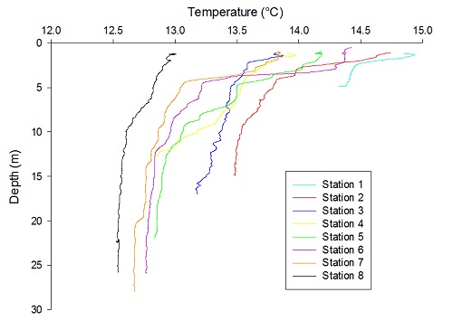
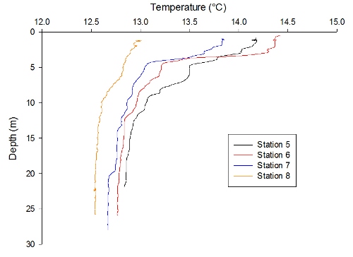
In general, from figure, there seems to be lower temperatures in the more southern
stations closer to the mouth of the estuary. This is reinforced when looking at the
contrast in temperatures from Stations 1 and 8: there is approximately a 2 °C difference
in the surface temperatures between these two sites. A clear thermocline is present
at approximately 5m depth with the largest ranges of vertical temperatures with depth
being in the mid-
Salinity
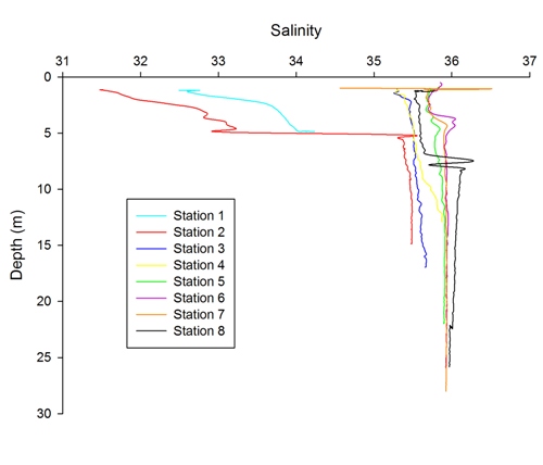
As seen from figure, there are higher salinities further towards the mouth of the
estuary. Haloclines are only noticeably present in Stations 1 and 2, with the lowest
salinity (approximately 31.5) being seen in Station 2. The largest range of salinities
with depth can clearly be seen in Station 2; this could be due to the high influx
of freshwater at Station 2. As freshwater is less dense than higher salinity water,
and so floats closer to the surface, this could explain the high jump in salinities
below the thermocline. Station 1, though further away from the mouth of the estuary,
may not be subject to as higher freshwater input than Station 2, and so has relatively
higher salinities in the surface layers. The haloclines are roughly at 5m depth,
which corresponds to the thermocline depths. The fluctuations in surface salinities
in Stations 3-
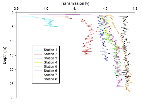
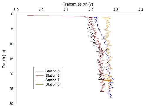
Transmission
It is clear from figure that the level of transmission increases further towards the mouth of the estuary, with Station 8 having the highest transmission value of approximately 4.7V. Though the levels of transmission fluctuate throughout the water column, Stations 1 and 2 in particular have much lower transmission values, especially in the surface. This could be due to Stations 1 and 2 locations: being further up the estuary, both stations have lower depths and a higher freshwater input from rivers. Not only do rivers bring suspended sediment into the estuary, but a shallower depth would mean that mixing would stir up the bottom sediment. Therefore, there is a higher percentage of suspended particulate matter (SPM), which would cause a lower rate of transmission. The opposite is true for the stations nearer the mouth of the estuary, particularly Station 8, which is located at Black Rock.
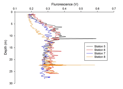
Fluorescence
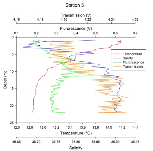
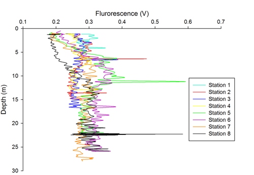
Fluorescence shows a general increase with depth over all stations (figure). Station 2 indicates a fluorescent spike at ~7m, station 5 spikes at ~11m and station 8 spikes at ~23m. With fluorescence being a proxy for phytoplankton these spikes may indicate a high number of phytoplankton at these depths. Other stations show some smaller spikes but not of substantial magnitude. As the station numbers increase the distance from the top of the estuary also increases, indicating that there are spikes of fluorescence at increasing depth toward the mouth of the estuary.
ADCP
ADCP data has been used to build up a picture of the backscatter in the water column which is an indication of phytoplankton and zooplankton presence. The Richardson’s number have been calculated from the flow data in order to work out the flushing rates of the estuary and to look at the flow patterns horizontally across the estuary.
Station 1-
Figure shows a broad lack of uniformity regarding backscatter at station 1. There are no bands of constant backscatter, with the values of backscatter ranging from close to 0Db and maximums of near 1Db. The chaotic appearance of this transect may be due to a very turbulent water column in a state of flux. It is also possible that as this was the first transect, the instruments may not have been set up correctly. Station 2, represented by figure, shows more uniform features when compared to station 1. The overall backscatter levels are low with values mainly below 0.5Db. This is likely a reflection of low levels of zooplankton and other large particles in the area. This trend of low overall backscatter is continued at station 3 (figure). However there is an area toward the east of the estuary that shows high backscatter intensity throughout the water column. This is likely either anomalous or a very local addition of large suspended particles which has not dispersed, the latter of which is highly unlikely. Due to station 4’s position in the northern half of the estuary, the backscatter values are continuing to reach a maximum of ~0.5Db (figure). The west of the estuary shows slightly higher backscatter intensity than the east of the estuary and could possibly be due to the influence of a creek in the area.
Station 5-
As seen in figure, the transect across the width of the estuary by Station 5 shows no clear maximum of backscatter. Below 2.5m, the backscatter is fairly uniform throughout the water column; however there is a slight minimum at 5m of about 62dB, possibly a result of increased turbulence. Areas of high backscatter are spread across the surface readings, likely to be a result of boats moving around the estuary or a higher volume of suspended sediment in the water from the outflow of the rivers. The transect across the width of the estuary by Station 6 (figure) again shows areas of high backscatter (around 84dB) across the surface readings, more so than at Station 5. This could be a result of more suspended sediment being transported into the estuary at this point by Mylor Creek. The sediment would be nearer to the surface at this point because it is being transported by freshwater, which is less dense than saline water, and so is on top. There are less spots of high backscatter towards the surface in the transect from across the width of the estuary by Station 7 (figure). This could be because there is no new input of freshwater at this point, so the water is better mixed and the sediments have dissipated throughout the water column. The few places with backscatter values of 109dB could be due to large fish, dolphins, or other such objects in the water. There is a slight increase in backscatter on the left side of the deep channel to about 79dB which could be due to flow. The backscatter seen in Station 8 (figure) is fairly uniform at around 67dB, with only isolated spots of higher backscatter where fish or other large, solid objects have crossed the path of the transect.
Flushing Time
Flushing time of the estuary was calculated using both the freshwater fraction and tidal prism methods. The tidal prism method was calculated using measurements of the estuary via Google Earth, navigational chart data and tide table data relevant to the 1st of July 2013. This method estimated the flushing time of the estuary for the 1st of July to be 5.59 hours. In comparison, the freshwater fraction method estimated the flushing time to be 104 hours. However due to the large amount of unavailable flow data for the majority of rivers that influence the Fal estuary, this method is likely flawed. A small value for R (freshwater flow volume) causes the resulting flushing time to be larger and this case to disagree with the tidal prism method. Due to the Fal estuary being a tidally dominated estuary and it experiencing spring cycles on the 1st of July, the tidal prism method’s flushing time is more likely value, despite being much smaller compared to the freshwater fractions method.
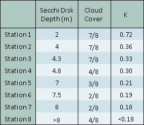
Attenuation Coefficient
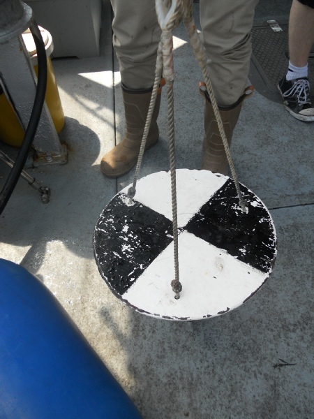
The attenuation coefficient generally decreases from the top of estuary toward the mouth. This is due to greater levels of turbidity in the upper estuary from riverine influence. Due to the limitations of the CTD aboard the RV Bill Conway, measurements of turbidity were not recorded. However the trend observed in the offshore activity suggests that turbidity increased toward the mouth of the estuary, it can be assumed that this trend continues up the estuary body itself. The CTD also did not allow for measurements of irradiance and so coefficients were only calculated using Secchi disk data. This data also has its limitations; at station 8 the rope on the Secchi disk was not long enough to get a precise Secchi depth.
Zooplankton
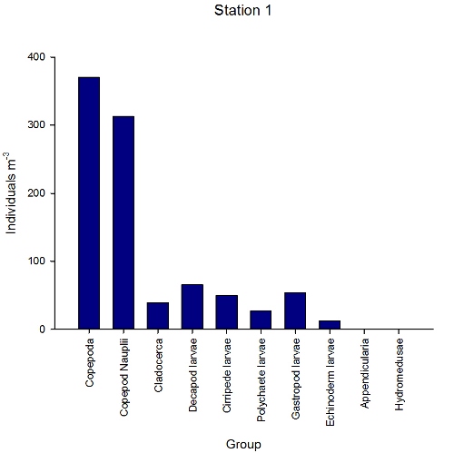
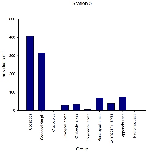
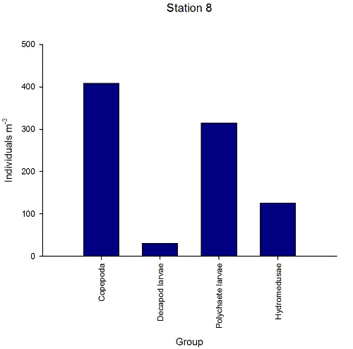
Station 1 (figure) at the top of the Fal Estuary and Station 5 (figure) in the centre are both comparable in terms of the species found and the total abundances. Station 8 (figure) at Black Rock had fewer species, but the total abundance of individuals was similar. Both stations 1 and 5 had high abundances of copepod nauplii. Previous studies into calanoid fecundity in the Western Channel have shown that females produce high volumes of small eggs during periods of high food availability, during the spring bloom for example (Pond et al, 1996). Phytoplankton cell counts in the estuary, particularly of the diatoms Chaetoceros and Nitzchia, were fairly high (table), as were the chlorophyll concentrations, particularly at station 5 (figure). It is possible therefore, that the high numbers of copepod nauplii observed were due to the nutritional content of the estuary.
Phytoplankton Species
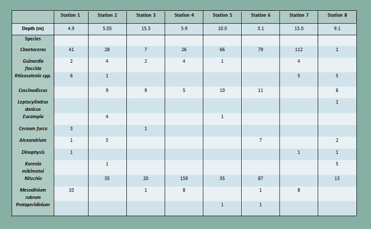
Samples for phytoplankton species distribution were taken from only one depth at
each sampling station in the Fal Estuary. In all cases, diatom species were found
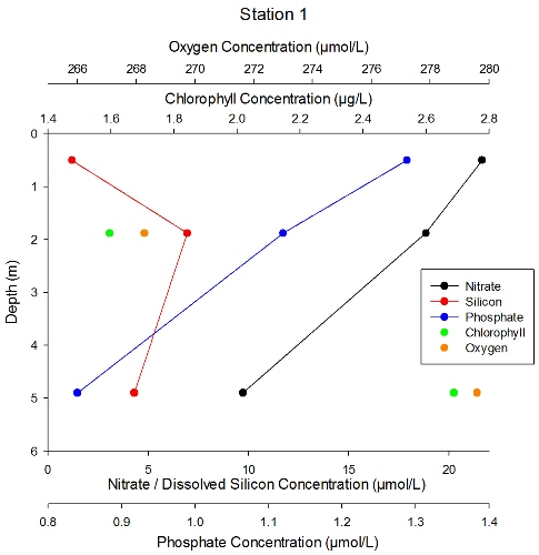
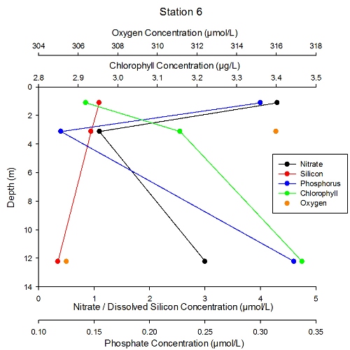
at these depths (table). At station 1, the silicon concentration increased between
the surface and 2m, and decreased between 2m – 4.9m (figure). This may suggest either
a high silicon input at the surface, or little diatom growth in the top 2m of the
water column. The concentrations of nitrate and phosphate both decrease between the
surface and 4.9m however, which may suggest growth of non-
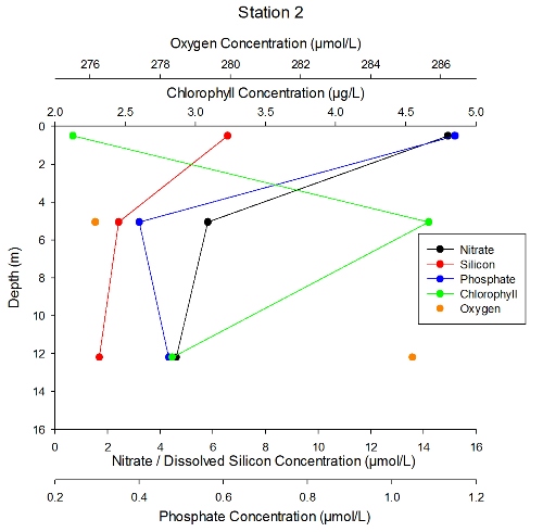
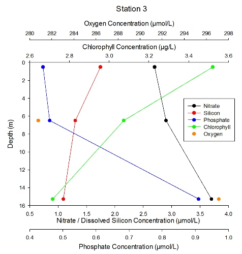
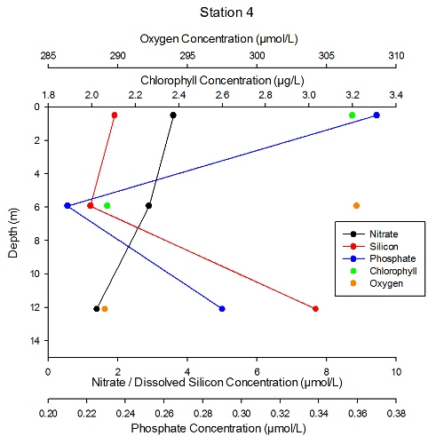
At stations 2 (figure), 3 (figure), 4 (figure) and 6 (figure) dissolved silicon concentrations were found to decrease between the surface and the sampling depth, as would be expected in areas with diatom growth. Dissolved silicon concentrations then increased below this depth at station 4, suggesting limited diatom growth. At stations 2 and 6, silicon concentrations continued to decrease slightly with depth, suggesting further diatom growth, although at station 2, overall chlorophyll concentrations decrease below ~5m, so the growth may not be extensive. Similarly at station 3, the overall cell abundances of all species found was fairly low in comparison to other stations, and the profiles of nitrate and phosphate suggest that phytoplankton growth is limited.
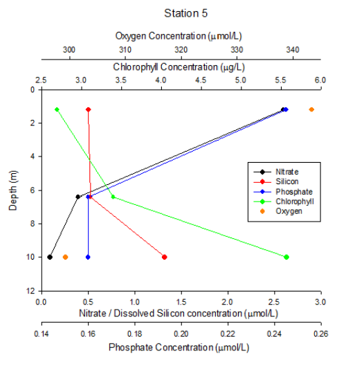
The phytoplankton species found at station 5 were primarily diatoms. Interestingly, dissolved silicon concentrations increased slightly between ~6m and the sampling depth of 10m, having remained constant above this depth (figure). It is possible that the diatoms that appeared in the sample had grown above 6m depth and then sunk to 10m. The stations in the centre of the estuary had slightly more stable water columns, and it has been suggested that for large cells to remain suspended, a certain amount of turbulence is needed (Kiørboe, 1993).
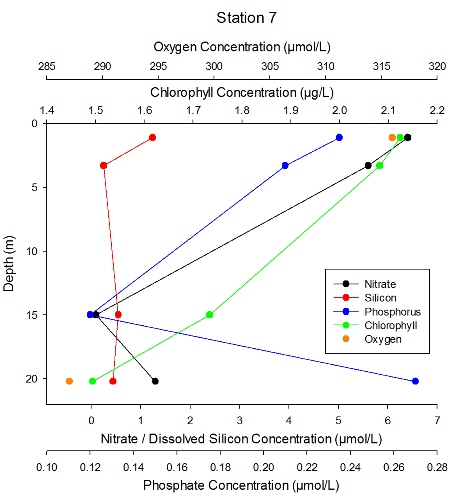
Station 7 exhibited a sharp decrease in dissolved silicon in the top 3m of the water column, perhaps indicating diatom growth (figure). The concentration remains relatively stable between 3m and the sampling depth of 15m, where there were particularly high numbers of Chaetoceros cells (table).
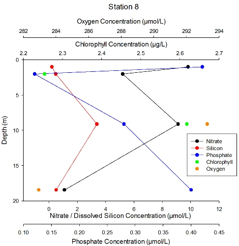
At Station 8 (Black Rock) both siliceous and non-
The majority of samples were numerically dominated by the diatom Chaetoceros. These findings are in line with previous studies of the phytoplankton communities of the Western Channel, which also noted that spring/summer communities were typically dominated by chain forming centric diatoms (Widdicombe et al, 2010).
Summary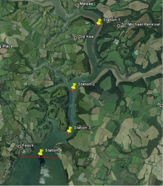
Water temperature and transmission were found to be lower at the stations located
towards Black Rock due to increased depth whereas salinity was found to be higher
at these stations. Fluorescence tends to increase with depth at all stations. There
appears to be no defined vertical backscatter pattern found by the ADCP transects
across most stations; however, at some stations such as 6, surface backscatter is
higher. The backscatter values increase from station 1 to 8. Due to the 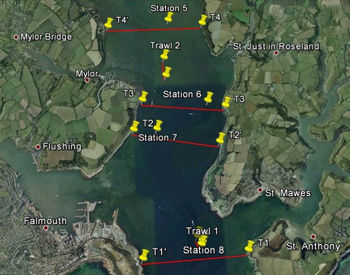 increased
turbidity in the upper estuary the attenuation coefficient decreased from here down
to Black Rock. Nitrate, dissolved silicon and phosphate show variability with depth
at all stations with concentrations being controlled by riverine inputs and phytoplankton
abundance. The TDLs show that all nutrients behave conservatively however phosphate
experiences addition in the upper estuary. At stations 1, 5 and 8 similar abundances
of zooplankton were found however at station 8 there were fewer species found. As
expected diatoms were found at all stations where dissolved silicon concentrations
were low. At Black Rock there was a mixture of diatoms and dinoflagellates were found.
increased
turbidity in the upper estuary the attenuation coefficient decreased from here down
to Black Rock. Nitrate, dissolved silicon and phosphate show variability with depth
at all stations with concentrations being controlled by riverine inputs and phytoplankton
abundance. The TDLs show that all nutrients behave conservatively however phosphate
experiences addition in the upper estuary. At stations 1, 5 and 8 similar abundances
of zooplankton were found however at station 8 there were fewer species found. As
expected diatoms were found at all stations where dissolved silicon concentrations
were low. At Black Rock there was a mixture of diatoms and dinoflagellates were found.
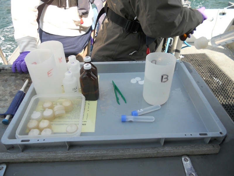
Sampling
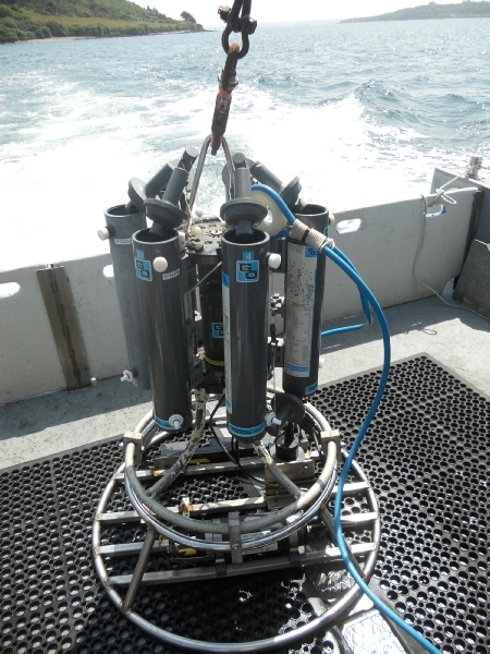
Whilst aboard the R.V.Bill Conway on the 1st July, 2013, samples were collected in
the Fal Estuary at 8 Stations, by groups 3 and 5. With the aid of a CTD, Niskin bottles
were fired at different water depths to analyse phytoplankton, dissolved oxygen,
nitrate, phosphate and dissolved silicon. With the use of a 100 µm plankton net,
with an opening diameter of 50 cm, two 5 minute horizontal trawls were undertaken
at Station 5 and 8. ADCP transects, across the estuary, were taken after visiting
each station, in order to obtain physical measurements. Due to the tidal state, with
high water at 1220UTC, 4.2m, and low water at 0621UTC, 1.3m, group 3 sampled Stations
1-
For chlorophyll sampling methods please refer to Chlorophyll. Sampling methods for phosphate, nitrate and dissolved silicon can be found in Nutrients.
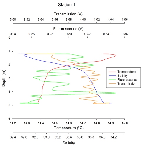
Station 1
Nitrate and phosphate concentrations were high at the surface and decreased substantially with depth. Concentrations were highest at the surface due to river inputs delivering the nutrients to the estuary. This agrees with the salinity profile, which shows lower salinity water sitting on top of higher salinity water. Dissolved silicon concentration was low at the surface and then peaked at ~2m in the water column, which may indicate the presence of diatoms near the surface, before decreasing again towards the bottom. The majority of the phytoplankton are between 4 and 5m, which can be seen from the chlorophyll and fluorescence trace (figure). Dissolved oxygen followed the same pattern as the chlorophyll, showing an increase with depth, which is due to the phytoplankton photosynthesizing and releasing oxygen into the water column.
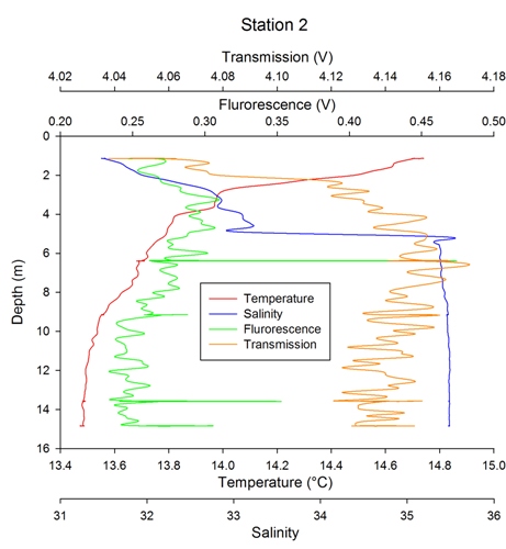
Station 2
Nitrate, phosphate and dissolved silicon concentrations are significantly higher at the surface and rapidly decrease to a depth of ~5m, though the concentrations were lower than at station 1 due to increased salinity. Concentrations are then mostly uniform for the rest of the water column. The chlorophyll concentration was quite low at the surface and then peaked at ~5m, coinciding with the CTD fluorescence measurements on figure; chlorophyll then decreased again throughout the rest of the water column. The peak of chlorophyll occurs at the same depth as the nutrient decrease, indicating that the phytoplankton at this depth were utilizing nutrients for growth. The decrease in dissolved silicon from the surface may indicate that diatoms were present in the water column. Dissolved oxygen increases with depth, which doesn’t follow the expected chlorophyll pattern.
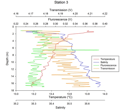
Station 3
Nitrate and phosphate concentrations increase slightly with depth, whilst dissolved silicon decreased slightly with depth (figure). Chlorophyll levels decreased with depth, indicating that there was slightly more phytoplankton at the surface. Oxygen levels increase with depth due to the input of denser, more oxygenation seawater from the lower estuary, transported inshore by the tide. As the nutrients increase only slightly with depth they are mostly constant throughout the water column. The phytoplankton could be depleting the surface nutrients and remaining at the surface to absorb more light for photosynthesis.
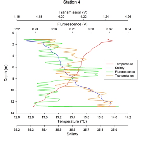
Station 4
Nitrate only decreased slightly throughout the water column (figure). Phosphate concentration was highest at the surface, decreased rapidly to ~6m and then increased again towards deeper depths. Dissolved silicon was fairly constant for the first 6m of the water column, but then a sharp increase occurred; this rise in dissolved silicon continued to the base of the water column. Dissolved silicon levels increased substantially between station 3 and 4; the map indicates 2 creeks between these stations which may have delivered more dissolved silicon to the estuary. Chlorophyll levels were highest at the surface and decreased substantially to ~6m. As silicon was depleted at the surface and chlorophyll levels were high at this point, diatom populations may have been present here. Dissolved oxygen concentrations were high in the middle of the water column and then decreased with depth; this is most likely due to less photosynthesizing phytoplankton being present in the deeper waters. CTD fluorescence data doesn’t appear to match the chlorophyll levels, but this may have been due to limitations in the data.
Station 5
Nitrate and phosphate concentrations are higher at the surface and then decrease rapidly with depth (figure). Dissolved silicon levels were constant from the surface to ~6m, before increasing with depth. Whilst chlorophyll levels increased with depth, nutrients decreased, indicating that the phytoplankton were utilizing and subsequently depleting the nitrate and phosphate. The increased chlorophyll levels at depth indicate that the phytoplankton were numerous at these points. Dissolved oxygen was higher at the surface, due to the high phytoplanktonic populations, and subsequently decreased with depth.
Station 6
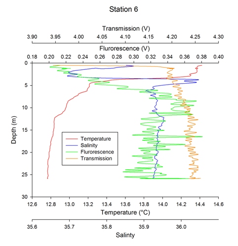
Nitrate and phosphate levels were high at the surface, and then decreased to ~3m before increasing to high levels again as depth also increased (figure). The levels of nitrate and phosphate increased between stations 5 and 6, which could be due to the multiple creeks adjoining the estuary between these stations. Chlorophyll levels increased with depth, indicating that majority of phytoplanktonic blooms were in deep waters; the phytoplankton populations at these depths most likely consisted of diatoms, as dissolved silicon concentrations deplete with depth, whereas the phytoplankton in surface waters are most likely smaller forms i.e. not diatoms, as the silicon is not depleted but the phosphate and nitrate are. Dissolved oxygen levels decreases with depth, which could be due to biological material near the seabed being decomposed by aerobic bacteria, which utilize oxygen as they respire.
Station 7
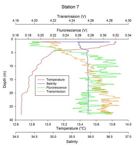
Nitrate and phosphate showed similar patterns to station 6. Dissolved silicon decreased slightly at the surface, from ~1.5µmol/L to ~0.5µmol/L, and then was fairly constant throughout the rest of the water column (figure). Chlorophyll levels were high at the surface before decreasing with depth, indicating that the majority of the phytoplankton were in the surface waters in order to utilize optimal levels of irradiance. The phytoplankton in the upper levels of the water column may be diatoms, due to the fact that dissolved silicon levels are limiting in most of the water column. However, closer to the bottom there may be other phytoplankton species, as indicated by the depletion of nitrate and phosphate at ~15m. Dissolved oxygen levels decreased with depth, which follows the chlorophyll pattern, and indicates that there are smaller populations of phytoplankton at depth that produce less oxygen from photosynthesis.
Station 8
Nitrate and phosphate levels were very high in the immediate surface, however, decreased rapidly in the first ~2m of the water column. Both then increased until ~8m, before nitrate decreased again with depth, whilst phosphate continued to increase. Dissolved silicon levels were low at the surface and at depth, but spiked around ~8m. Chlorophyll levels appeared to increase slightly around ~8m depth and the levels agreed with the fluorescence from the CTD (figure). The chlorophyll peak occurred when the nutrient levels were relatively high which suggests that maybe light was limiting the phytoplankton growth. Oxygen appeared to decrease with depth and didn’t follow the predicted profile that matches chlorophyll.
Theoretical Dilution Lines
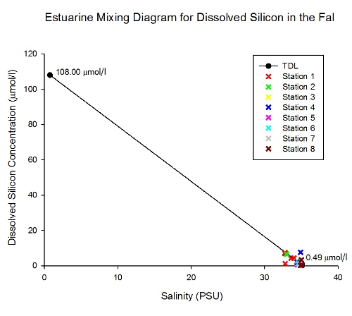
Dissolved Silicon
Figure indicates that dissolved silicon behaves conservatively in the estuary. Conservative
behaviour occurs when the concentration in the estuary is purely determined by mixing
processes. As the majority of the points follow the pattern of the theoretical dilution
line (TDL) it is conservative. There are some data points which are distant from
the TDL but not enough data points are different for it to constitute non-
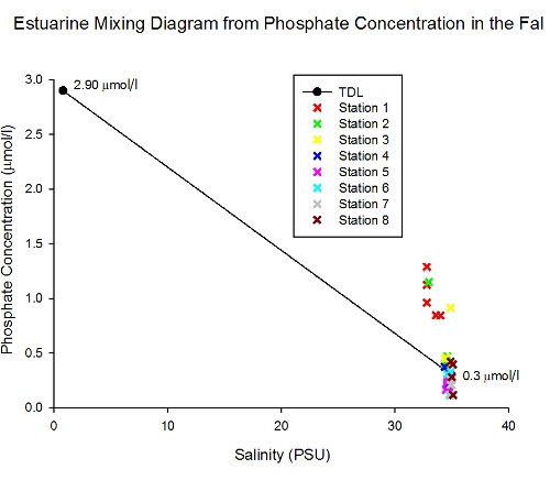
Phosphate
Phosphate shows mostly a conservative pattern in the estuary with its concentration being determined by mixing processes and not chemical processes. Phosphate concentration is higher at the top of the estuary and decreases with distance from the top of the estuary (figure). Riverine input is the main source of phosphate to the estuary. Station 1 data points are higher than the TDL which indicates non conservative behaviour with phosphate being added to the estuary at this station. This may be due to a higher than normal input of phosphate at this location such as run off of fertilizer. Some measurements from station 2 and 3 (quite close to the top of the estuary) are also higher than the TDL.
Nitrate
As seen in figure, nitrate concentration mostly shows conservative behaviour down
the estuary. As the points lie along the Theoretical Dilution Line (TDL), this shows
that the distribution of nitrate in the estuary is determined by mixing processes
(i.e. nitrate is conservative along the estuary). Similarly with the Estuarine Mixing
Diagrams for both phosphate and dissolved silicon, the concentrations of nitrate
are higher the lower the salinity is i.e. higher up the estuary. This is because
the further up the estuary, the more riverine and freshwater/agricultural run offs
are transported into the estuarine basin. Land run-

CTD
Station 1

Parameters
Stations 5-
Stations 5-
Stations 5-
Stations 5-
ADCP
Nutrients
Zooplankton
Station 1
Station 5
Station 8
Phytoplankton
Estuarine
Mixing Diagrams
| Activites |
| About Us |
| References |
| Physical |
| Chemical |
| Biological |
| References |
| Physical |
| Chemical |
| Biological |
| References |
| Poster |
| References |
| YSI Probe |
| Current Meter |
| Light Meter |
| References |