The aim of the study was to investigate the chemical and physical structure of the Fal estuary and its degree of mixing by collecting water samples and measuring the concentration of nutrients at various stations down the estuary. The Fal estuary has an unusual distribution of nutrients and a changing flow dynamic throughout. Therefore another aim was to understand the phytoplankton and zooplankton community dynamics at different stations along the estuary with respects to these properties.
At a station several factors were measured, this included:
- The flow regime was visualised using an ADCP which measured the current velocities along a transect, from one side of the river to the other.
- A CTD rosette was deployed to provide a preview of the water column. Niskin bottles were closed at selected depths according to specific sections of the water column. This could be when a parameter was changing significantly with depth. These samples were then analysed to obtain a representation of the properties of the water column at that location and were preserved in separate bottles to be analysed at a later date in the lab. Concentrations of chlorophyll, nitrate, phosphate, silicon will be calculated and phytoplankton and zooplankton observed, identified and compared.
The methods used to preserve the water samples for each parameter can be seen in the methods section of ‘Offshore’.
ADCP
Data was taken from stations 1, 2, 3 and 4 on a rising tide, whilst stations 5, 6,
7 and 8 were taken on a falling tide. This tidal pattern is reflected in the average
current readings from the ADCP. At station 3, where the river channel flows from
east to west, the ADCP transect shows a strong eastward flow at depth, where dense
sea water on the rising tide undercuts the less dense fresh water. At station 4 (fig.1),
there is evidence of a landward flow at approximately 6-
FLUSHING TIME CALCULATIONS
Tidal flushing of the estuary will result in a Flushing time T, of approximately:
Ttidal= 12.42 hours (tidal period)
Vestuary= 1.36×10⁷m3 (Volume of Estuary=mean area× mean depth, the mean depth is 10m, which makes the area 1.36×10⁶m2.)
Vprism= Area of estuary × h (tidal range) = 1.36 × 10⁶ m2 × 3.4m
h= (average of spring and neap tidal range) =3.4m
T= 1.5 days.
Station 1(fig. 3 & 4)
Dissolved silicon appears to be depleted (1.17µM) in the surface waters where there is an indication of diatoms, but dissolved silicon increases at 2m depth. All nutrients show a lower concentration at the base of the profile than at 2m depth, due to being utilised in overlaying water. Dissolved oxygen shows super saturation at 111.8%, due to the mixing of the water column. Chlorophyll concentration is also higher at the middle of the water column, where light levels are higher although variation throughout the water column is lacking ultimately due to the shallow depth of this station, the small variation is reinforced within the CTD profile. The water column is separated by the thermocline, due to warmer fresh water and cooler salt water intrusion throughout.
Station 2 (fig. 5& 6)
At station 2 dissolved silicon, phosphorous and nitrate all follow similar patterns, decreasing quite dramatically in the first 5m of the profile. This is consistent with the chlorophyll patterns which remain approximately constant around 3.164mg/l for the first five metres, and decrease significantly after this. Dissolved oxygen increases with depth, due to the higher biological presence at the lower depths depleting the oxygen within the water column. The calm surface conditions mean that limited oxygen would enter the water from the surface compared on days where conditions are likely to be more volatile and surface shear is greater. The flurometer and chlorophyll data do not appear to be correlated particularly well, with the flurometer only registering a spike just deeper than 6m. The water column is vertically stratified due to warmer fresh water at the surface and cooler salty water below the mixed layer.
Station 3 (fig. 7 & 8)
Dissolved silicon concentrations continue to decrease with depth. Chlorophyll concentrations appear to peak at the surface with values of 3.521µM, but the flurometer indicates a peak in chlorophyll between 6m and 7m. This is equitable between available nutrients of phosphate and nitrate, as well as oxygen with the surface light availability. Dissolved oxygen follows the previous station trend.
Station 4 (fig. 9 & 10)
Dissolved silicon concentrations change similarly to other stations, with the base
of the water column having a higher concentration. Phosphate and nitrate decrease
with depth, as they are utilised by the phytoplankton present. Chlorophyll and flurometer
data contrast each other at this station, so if it were possible, these samples should
be re-
Station 5 (fig. 11 & 12)
Dissolved silicon, phosphate and nitrate all decrease in concentration with depth alongside dissolved oxygen. There are considerable differences in dissolved silicon at this station compared to previous stations (silicon concentration at depth for station 4 is 7.69µM whilst at station 5 it is 0.42µM) this gives evidence that diatoms are present between these stations and are utilising the silicon. This is reflected in the increasing chlorophyll and flurometer readings from the surface to the seabed.
Station 6 (fig. 13 & 14)
Dissolved silicon is depleted homogenously throughout the water column, whilst phosphate and nitrate decrease rapidly in the upper 3m but increase at the seabed with a maximum 0.33µM and 2.99µM respectively. Chlorophyll and the flurometer readings indicate increased phytoplankton below the thermocline at approximately 3.3m at 2.12mg/l. This pronounced thermocline is likely to be emphasised by the sunny conditions that allow for strong stratification to occur.
Station 7 (fig. 15 & 16)
Silicon at this station decreases rapidly in the surface layer, and remains in low
concentrations down to 0.252µM compared to the riverine end members with an average
value of 108µM. Phosphate concentrations appear relatively unaffected by chlorophyll
concentration changes. As expected, nitrate varies inversely to the flurometer readings
and chlorophyll concentrations. Dissolved oxygen decreases as the depth increases,
due to organisms consuming oxygen throughout the water column to facilitate metabolic
respiration. The thermocline seen at 5m depth correlates to an increase in chlorophyll
concentration as nutrients from the sub-
Station 8 (Black rock)(fig. 17 & 18)
Dissolved silicon increases in concentration until 9.1m depth, where dissolved silicon peaks at 3.382µM at the base of the thermocline, then decreases to surface concentrations at 19m. Phosphate is depleted rapidly from 0.42µM at 1m, down to 0.12µM at 2m, and then increases with depth to values similar to those at the surface (0.40µM at 18.45m). Nitrate follows a similar pattern but is depleted from the water at approximately 18.45m depth, and covers the same range of concentrations seen at the northern end of the estuary.
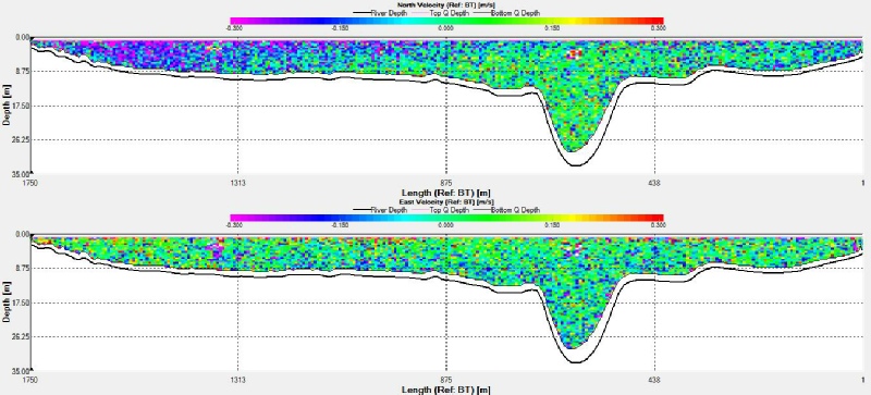
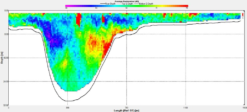
Fig.1 ADCP transect across the Fal estuary at station 4 showing velocity in a longitudinal axis
Fig.2 ADCP transect showing backscatter at station 7 longitudinal axis
Click on image to enlarge
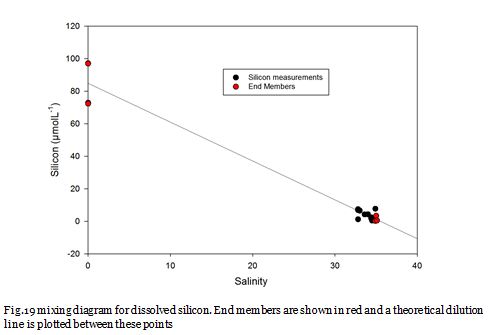
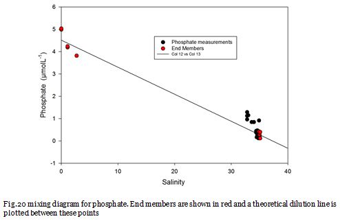
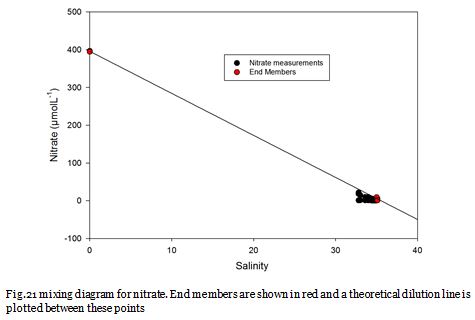
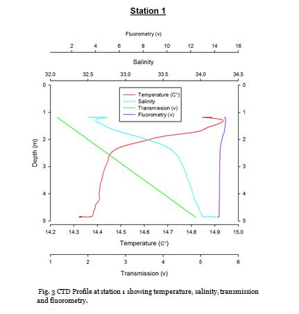
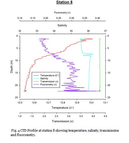
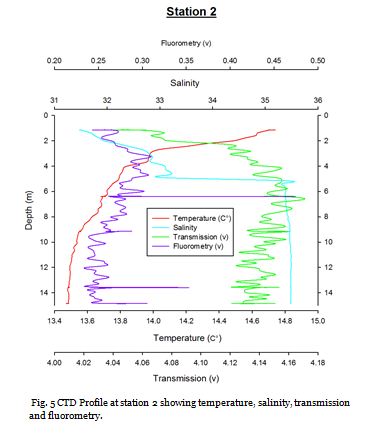
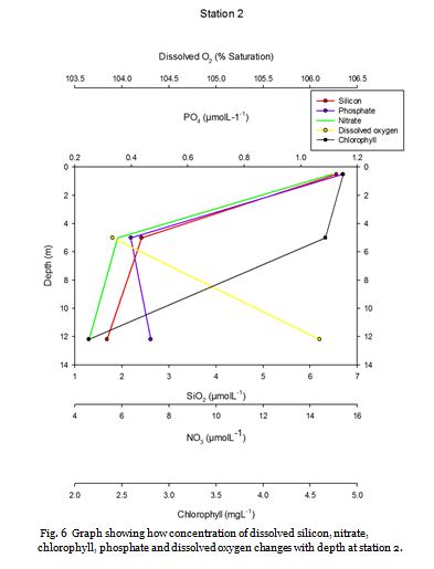
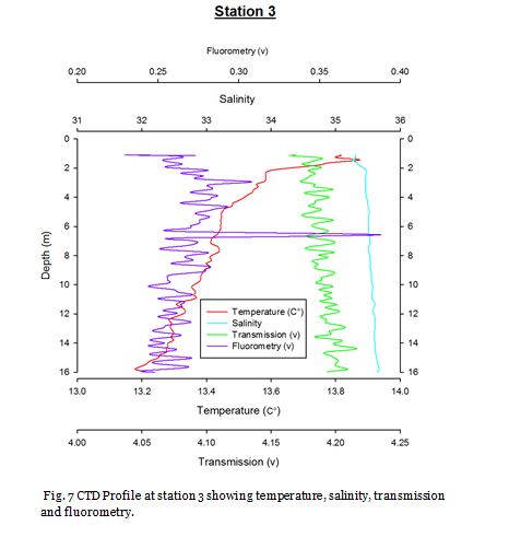
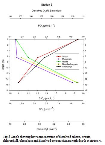
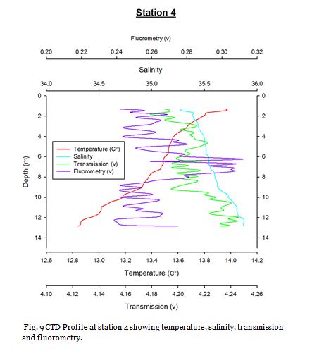
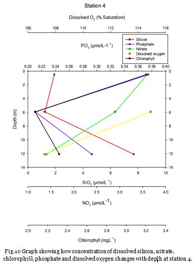
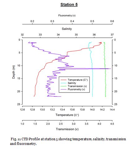
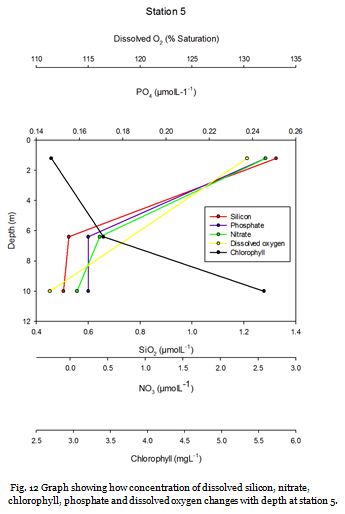
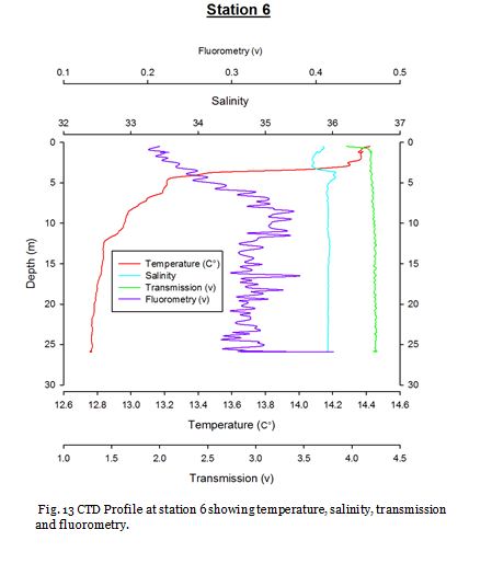
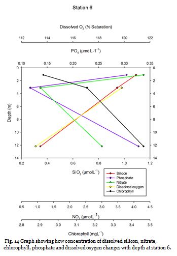
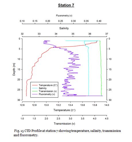
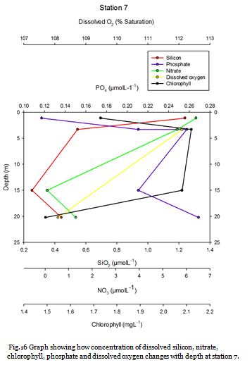
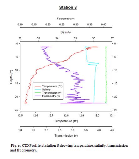
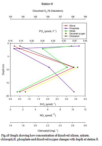
Fig.3
Fig.4
Fig.5
Fig.6
Fig.7
Fig.8
Fig.9
Fig.10
Fig.11
Fig.12
Fig.13
Fig.14
Fig.15
Fig.16
Fig.17
Fig.18
Fig.19![]()
Fig.20
Overall
Oxygen % saturation rates are fairly constant throughout the estuary, whilst other
elements are depleted. Dissolved silicon decreases significantly between station
4 and 5, which could signify a diatom bloom between these stations. Nitrate levels
are at their lowest mid-
Mixing Diagrams
The mixing diagrams produced for silicon (fig. 19), phosphate (fig. 20) and nitrate
(fig. 21) can be used to determine whether the mixing was behaving conservatively
or non-
The silicon mixing diagram shows a theoretical dilution line supporting a higher
concentration of dissolved silicon towards the riverine end member, as would be expected.
However the water that was sampled only decreased to a salinity of 32.8 and therefore
the mixing diagram cannot be used to decipher whether the dissolved silicon was acting
conservatively or non-
Phytoplankton:
Chaetoceros increases from station 4 to 7 (fig. 22) with a peak of 1120 cells ml-
Zooplankton
Adult copepods and nauplii made up the vast majority of the zooplankton community
at Station 1 (fig. 23) and 5 (fig. 24). Station 8 (Black rock, fig. 25) is notable
in that no nauplii were recorded, which is surprising due to the high abundance of
adult life stages. Polychaete larvae were found at all three stations, although the
highest numbers were taken from Black rock (314 ind. m -
Click on image to enlarge
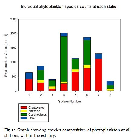
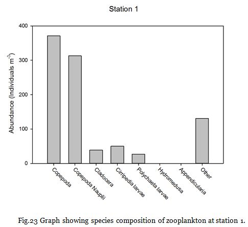
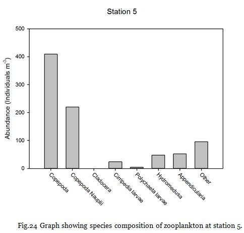
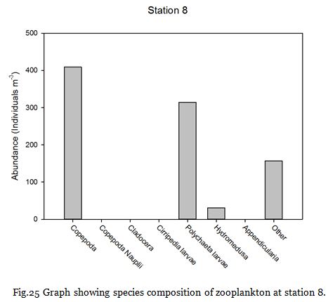
Fig.22
Fig.23
Fig.24
Fig.25
There are several limits associated with the estuary practical that we undertook.
A major limitation was that we split the sampling between groups 3 and 5. Inconsistencies
with the sampling methods that were undertaken could have influenced results that
we obtained, alongside a significant time delay where groups changed over. Limited
bottle sampling also means that at all stations phytoplankton was sampled only once,
and the zooplankton was only trawled at 3 stations -
Fig.21
Disclaimer: The opinions and conclusions expressed in this website are not affiliated with those of the National Oceanography Centre or the University of Southampton.
| Introduction |
| Methodology |
| Physical analysis |
| Chemical and phytoplankton |
| Zooplankton |
| Introduction |
| Methodology |
| Side-scan |
| video transect |
| Limitations |
| Poster |
| Introduction |
| Methodology |
| Results |
| Limitations |
| Introduction |
| Methodology |
| Physical analysis |
| Chemical analysis |
| Biological analysis |
| Limitations |