Group 2 Plymouth Field Course


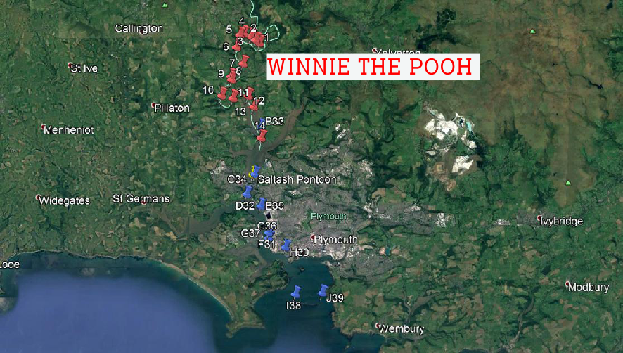
On 7th July, we collected data from the Tamar Estuary in three different sections. One group went on the Falcon Spirit and collected data up the estuary until Calgreen (shown on the map below). Another group went on the Winnie The Pooh and sampled further up the estuary. A final group went to Salt Ash Pontoon and took a time series throughout the day. Click on the location on the map below to see the data collected from these different locations.


ESTUARY
Station Locations


Salinity Gradients


Zooplankton


Phytoplankton
Fig 1 -
Fig 2 -
Fig 3 -
Fig 4 -
Fig 5 -


Fig 6 A -
Fig 6 A -
For each Zooplankton sample taken, Copepods dominate the populations (fig 4). At station H30 the sample analysed found 168 Copepods and 196 Copepod naupliia per m3 of sea water (fig 4e). Station D32 had an estimated 54 Copepod individuals per m3 of sample (fig 4d). Station I38 had a much smaller density of zooplankton, with only an estimated 3 individuals per m3 of sample, 1 of which was found to be a Copepod (fig 4f.), compared to 523 individuals per m3 at Station H30. Station I 38 was by the Plymouth break water, where as H20 and D32 were further up the estuary. This difference in location could be the cause in the difference in zooplankton density. The Plymouth break water prevents mixing so surface waters are nutrient limited and with the high temperatures, stratification of the water column will be increased by strengthening the thermocline, preventing mixing. Further up the estuary the water will be more mixed, due to it nearing high tide when samples were taken, distributing nutrients in the water column. The nutrient TDL’s showed that as soon as the salinity reached 34/35 (off shore) nutrients fell out of the water column (see estuary TDLs section) , indicating there is less nutrients available so only smaller populations can be sustained. More predation could have occurred towards the sea rather than in the estuary due to only limited species being adapted to the fluctuating salinities. Species were less diverse at I38 compared to the estuary site. This area could be more susceptible to predation due to the sea and the river meeting. All had fish larvae, indicating the lower estuary could be a nursery ground for some species
Further up the estuary, Copepods still dominate the zooplankton population. Station 1 had 107 copepods per m3 of sample (fig 4a), station 6 had 847 copepods per m3 (fig 4b) and station 14 had 1675 copepods per m3 (Fig 4c). Decapod larvae were also found at each station. Species diversity was similar between stations, but zooplankton density varied greatly. Station 1, which was the highest station up the estuary, had a count of 143 individuals per m3 compared to station 14, which was further down the estuary, had a count of 1692 individuals per m3. This could be caused by predation by fresh water species. Further down the estuary, the fluctuating conditions create a harsh environment with few species enable to survive in these conditions, so perhaps less predation occurs here. The low phytoplankton levels further up the estuary will influence the number of zooplankton, due to being a food source.
Phytoplankton density varies across sample sites. The stations near the break water have higher population densities, with station J39 having 321 cells per ml compared to stations C34 having 13 cells per ml (fig 5). This is probably due to high turbidity occurring in the estuary compared to the sea, limiting the phytoplankton growth, even though there are high concentrations of nutrients in the estuary compared to near the breakwater (See TDLs). Grazing pressure by zooplankton will have also affected phytoplankton densities, with zooplankton populations greater towards the estuary than out by the break water. Diatoms dominated throughout the stations, with Chaetoceros counts reaching 162 individuals per ml of sample at station H30 (fig 5). Phytoplankton species were more diverse towards the lower estuary and break water (Fig 6) compared to the number of species found up the estuary. This may be because the pressure for nutrients is high in this area, enabling more species to dominate new niches. Previous research has found phytoplankton species richness declined with increased nutrient levels (Leibold, 1999).
Further up the estuary, phytoplankton density varied between sites once again. Station
1, the station furthest up the river, only had 4 cells per ml of sample, compared
to station 14, further towards the estuary, with 628 cells per ml of sample (fig
6). This is probably due to increased turbidity up the estuary, it was noted when
analysing station 1 samples, there was a lot of dirt in the sample, which would not
be ideal for photosynthesis and growth of phytoplankton due to low light levels.
Diatoms dominated throughout the samples, with counts reaching as high as 140 cells
per ml at station 14 (fig 5). Diatoms require less energy to form in comparison to
other shell forming phytoplankton and so out-
References
Leibold., M., A., (1999). “ Biodiversity and nutrient enrichment in pond plankton
communities”. Evol. Ecol., Res 1: 73-
Raven, J. A. (1983). “The Transport and Function of Silicon in Plants”. Biol. Rev.,
58. pp179-
Lui, H. and Chen, C. (2012). The nonlinear relationship between nutrient ratios and salinity in estuarine ecosystems: implications for management. Current Opinion in Environmental Sustainability, 4(2), p.1.
Morris, A., Bale, A. and Howland, R. (1981). Nutrient distributions in an estuary: Evidence of chemical precipitation of dissolved silicate and phosphate. Estuarine, Coastal and Shelf Science, 12(2), pp.209
Statham, P. (2012). Nutrients in estuaries — An overview and the potential impacts
of climate change. Science of The Total Environment, 434, pp.213-
The views and opinions expressed are those of the individual and not representative of the University of Southampton or the National Oceanography Centre.
Temperature was plotted against salinity and depth. Salinity was used as a conservative
measure of the river-
The actual data points are indicated by squares on the contour graph. Therefore,
the temperatures that fall away from these points have been generated by the software
and do not represent samples, so cannot be assumed to be accurate. For example, where
salinity was less than 16, the maximum depth was only 4m -
Regardless, the contour graph is still indicative of the major trends, and is a useful tool in visualising this. It is clear that the warmer surface waters has been heated most extensively by the sun to up to 23.5˚C, whilst the deeper (beyond 3m), saltier (above 30 psu) water intruding from the ocean is much cooler, down to 19.5˚C
This contour graph shows the salinity changes in the vertical and horizontal directions for the Tamar estuary. Salinity is used one more time as the independent variable.
The rising graph represents a transect that describes a partially mixed estuary, where the river input is being subjugated by a tidal input. This is shown by the evenly distributed isohalines sloping towards the head of the river (where salinity is 0 psu); fresh, lighter water sits on top while salty water relies at the bottom creating a frictional gradient that turns into turbulence and eventually mixing, pushing the isohalines towards vertical profiles.
Observing a correlation with the temperature contour, the tidal input is clearly detected by its high salinity (32.6 psu) and low temperature. Likewise, the riverine endmember is spotted sitting at the first and highest station with a salinity of 6.8 psu.
Figure 3 shows surface concentrations of the nutrients silicon, phosphate, nitrite and nitrate across a transect of the Tamar Estuary, starting at a salinity of 7 near Calstock and becoming more saline up to the confluence of the rivers Tamar and Tavy. Overall, there is generally decrease in the total nutrient concentration as salinity increases. The riverwater has a high nutrient load due to weathering of rocks in the river’s catchment, which are then removed along the estuary by processes such as biological uptake, flocculation and coagulation so by the time it reaches the estuary mouth, the water column is depleted in nutrients as seawater generally has a low nutrient concentration (Lui and Chen, 2012). In contrast, there is a sharp increase in phosphate concentration at the confluence at a salinity of 33, suggesting a new input of this nutrient (Morris, Bale and Howland, 1981). The dominant nutrient in this estuary is nitrate, which is expected as this is the more stable form of nitrogen in oxic conditions (Statham, 2012) and can often have high anthropogenic inputs due to processes such as agricultural runoff and sewage treatment ((Lui and Chen, 2012).
Figure 3 also shows surface concentration of the pigment chlorophyll with increasing salinity along the Tamar estuary. The trend shows an overall decrease, although this fluctuates greatly with a sharp increase at around salinity 16 – this corresponds with a sharp increase in nutrient concentration at this salinity shown . Chl a is often used as an indicator of presence of phytoplankton, suggesting that this increase may be due to an increase in essential nutrients available to the plankton. The overall decrease is likely to correspond to the depletion of nutrients with increasing salinity, as there are less available in the more saline water to facilitate phytoplankton blooms.


