Group 2 Plymouth Field Course

ZOOPLANKTON

PHYTOPLANKTON

BIOLOGY

A plankton net was lowered over the side of the boat with a collection bottle attached to the end. The net was raised through a chosen depth and the sample was collected. 1 litre of this seawater was set in formalin. 10 ml was measured out for each repeat. 5 ml at a time were pipetted into a Bogorov chamber and the amount/species of zooplankton were counted using a microscope. This process was repeated for all the samples. Then the number of zooplankton per m³ was calculated using the number of zooplankton in a 10ml sample and the volume of sea water sampled. The volume of seawater sampled can be calculated by the equation: ,where R is the radius of the plankton net opening, L is the distance the net was towed and V is the volume.

The depths sampled on the Callista were 0-20m and 20-40m at site C5 and 0-20m at site C4. Below, the data for these sites has been presented as pie charts of the number of each species per m³ of seawater with their corresponding temperature and salinity depth profile.

Seawater is collected at chosen depths in Niskin bottles on a CTD rosette. 100 ml of each sample was collected and 1 ml of iodine was added to kill the phytoplankton cells. The sample was left overnight so the phytoplankton could bind to the reagent and settle to the bottom and it was then stained with Lugol's iodine. The top 90 ml of seawater was removed using a vacuum pump to leave a concentrated 10ml sample. 1 ml of this solution was then pipetted onto a slide and placed under a microscope. The amount and type of species was recorded for 100 squares. This number is then multiplied by 10 to give the phytoplankton count per ml

The zooplankton count for C5 0-20m of the water column (Figure 2B) demonstrate that Echinoderm larvae were most abundant form of zooplankton in surface waters with 9 individuals per 10ml of sea water. Echinodermata have been found to be one of the most abundant forms of meroplankton in the Plymouth Sound following phytoplankton blooms (Highfield et al., 2010).
Between 20-40m the species diversity increases compared to zooplankton counts above 20m (figure 2C). Plotting the temperature shows that the thermocline is present at 20m in the water column. Perhaps the species diversity increased due to the increased particulate matter collecting below the thermocline due to export from above. Research has found that the thermocline can influence the spatial distribution and composition of zooplankton (Cantin et al., 2011). Species that dominate this region included Cirripeda and Copepoda taxa, with 16 and 12 individuals per 10 ml of seawater retrospectively. Cirripeda have been found to dominate Plymouth sound zooplankton communities and the high abundance of copepod sp. was expected as they are considered one of the most common metazoans and are crucial to the pelagic food web and microbial loop. (Nielsen and Richardson, 1989).

Fig 2 A - Station C5 temperature and salinity depth profile with the two plankton trawl depths (0-20m and 20-40m) shown.

Fig 2 C - Pie chart showing the ratio of each zooplankton species per m³ for 20-40m at station C5.

Fig 2 B - Pie chart showing the ratio of each zooplankton species per m³ for 0-20m at station C5.

Fig 1 A - pie chart showing the ratio of zooplankton species per m³ for 0-20m for station C4.

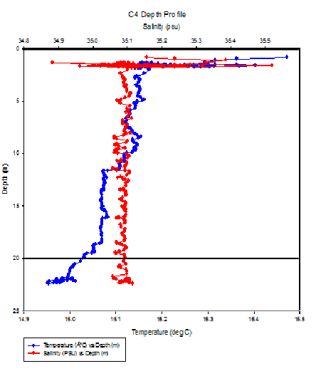
Fig 1 B - station C4 temperature and salinity depth profile with the plankton trawl depth shown

Table 1 - showing the average number of zooplankton per m³ for each sample

The zooplankton count for C4 demonstrates that Cirripeda and Copepoda larvae dominate the zooplankton community at this site (figure 1A) with 31 and 10 individuals per 10ml of seawater sample retrospectively. The temperature and salinity profile shows that the water was fairly homogenous above 20m where our sample was taken (figure 1B). C4 had a higher number of individuals per 10ml of sample compared to C5 samples, with 72 individuals compared to 66 and 11 per 10 ml. This difference could potentially be due to location, there may be increased nutrient inputs fuelling increased phytoplankton growth which can support a larger zooplankton community.

a

b

c

d

e

The of species diversity between stations but all were dominated by diatom species. C1 was dominated by Chaetoceros diatoms (Fig 4A). C3 had a greater variety of species but once again was dominated by diatoms, Chaetoceros chained diatoms in particular (fig 4b). The C4 sample only comprised of diatoms and dinoflagellates (fig 4c). C5 was dominated by Chaetoceros Psuedo-nitzschia diatoms and dinoflagellates (fig 4d). C6 also was dominated by Chaetoceros diatoms but also Phaeocystis colonies too (Fig 4e). Like C5, C7 was also more diverse but once again diatoms dominated. Due to their silica shells, diatoms are considered the most dominant species of phytoplankton in the Northern Hemisphere during the spring and summer blooms (Yool and Tyrell, 2003) . This is because require less energy to form in comparison to other shell forming phytoplankton and so out-compete other species (Raven, 1983). Phytoplankton blooms are usually successional and so perhaps the recent weather conditions and nutrient input favour diatoms growth.

The distribution of phytoplankton density suggests that phytoplankton abundance peaks at 20m (fig 3) for most stations. For example, C5 density peaks at 20m with 2510 cells per ml of sample compared to 410 cells per ml at 5m depth. C3 and C7 also show an increased density at 20m with cell counts reaching 1630 and 230 cells per ml retrospectively. C6 shows a decrease in density below 20m, from 1180 to 40 cells per ml, which may be due to insufficient irradiance to photosythesise and grow. The temperature and salinity profile showed 20m  was where the thermocline is (see offshore physics page). This peak of abundance at the thermocline suggest this is a Deep Chlorophyll Maximum Bloom. These are found globally in our oceans and are where the phytoplankton are able to access the nutrient rich waters below the thermocline but still have sufficient sunlight to photosynthesise (Huisman et al., 2006). The lack of sampling throughout the water column, particularly at stations C1 and C4 means that this theory cannot be confirmed at all the stations.

Phytoplankton density varied between stations (fig 5). C5 had the highest abundance with a total average cell count through the water column of 1540 cells per ml of sample. C4 had the lowest total average cell count, with only 50 cells per ml of sample. The variation in phytoplankton cell density could be caused by variation in terrestrial and riverine inputs, essential sources for nutrients needed for phytoplankton growth (Tyrrell, 1999)  and so can support a larger community. Stations 1-5 were near land and so will be more affected by terrestrial inputs, compared to stations C6 and C7 which were further out to sea. C6 and C7 would be more stratified due to their location, limiting nutrient supply and mixing, which explains their lower cell densities of 610 and 157 cells per ml of sample retrospectively. However this still does not explain why station C4 had low phytoplankton density. Only 1 sample was taken at this site and so perhaps more samples taken at a greater variety of depth may demonstrate increased phytoplankton growth a different depth.

Fig 3 - Phytoplankton density depth profile for all stations.

Fig 4 - Pie charts of the ratio of phytoplankton species density at all stations; a=C1, b=C3, c=C4, d=C5, e=C6 and f=C7.

f

Fig 5 - bar chart of the total phytoplankton density for each station

References

Cantin, A., Beisner, B., Gunn, J., Prairie, Y. and Winter, J. (2011). Effects of thermocline deepening on lake plankton communities. Canadian Journal of Fisheries and Aquatic Sciences, 68(2), pp.260-276.

Highfield, J., Eloire, D., Conway, D., Lindeque, P., Attrill, M. and Somerfield, P. (2010). Seasonal dynamics of meroplankton assemblages at station L4. Journal of Plankton Research, 32(5), pp.681-691.

Huisman, J., Pham Thi, N., Karl, D. and Sommeijer, B. (2006). Reduced mixing generates oscillations and chaos in the oceanic deep chlorophyll maximum. Nature, 439(7074), pp.322-325.

Nielsen, T. and Richardson, K. (1989). “Food chain structure of the North Sea plankton communities: seasonal variations of the role of the microbial loop”. Marine Ecology Progress Series, 56, pp.75-87.

Tyrrell, T. (1999). The relative influences of nitrogen and phosphorus on oceanic primary production. Nature, 400(6744), pp.525-531.

Raven, J. A. (1983). “The Transport and Function of Silicon in Plants”. Biol. Rev., 58. pp179-207.

Yool, A. & Tyrell, T. (2003). Role of Diatoms in Regulating the Ocean’s Silicon Cycle. Global Biogeochemical Cycles, 17(4)

The views and opinions expressed are those of the individual and not representative of the University of Southampton or the National Oceanography Centre.