Introduction

Map 1. Map displaying the location of each station sampled on the RV Callista on the 10/07/2017 ranging from station 30-37. The stations in progessive distance from the coastline; station C37 (0.33km from the coastline), station C36 (0.96km), station C35 (1.5km), station C30 (2.6km), station C34 (3.4km), station C33 (7.2km), station C31 (10Table 2. Table showing the coordinates and time of sampling (UTC) at each station (30-37) offshore. .6km) and station C32 (14.1km).

The purpose of the offshore surveying was to enhance our understanding of the spatial and depth structure of the water near the Falmouth estuary. Our focus was the deep chlorophyll maximum (DCM) and the presence of a potential double DCM layer; however, we did also look at nutrients and oxygen in the water. To investigate this, we deployed a CTD with several niskin bottles and then deployed zooplankton nets to collect physical samples at depths of interest. We first worked out far offshore with our first station being about 15 miles due south of the Falmouth estuary. From here we then worked due west towards the coast to see how this front changed as we progressed towards the coast.

A front is an area/location with two very different water masses. The front we were looking at involved the DCM where, once crossed, it was no longer visible and instead the water was more mixed than stratified. Each site was chosen so that we continued along a constant line and could see how the DCM changed as we approached the front, at the front and past the front. On the eastern side of the front we have two separate mixed layers and as we move west to the coast passing through the front these mixed layers compress due to decreasing depth. As a result they are forced to mix as one. This leads to a well-mixed coastal water.

Phytoplankton

The CTD’s Niskin bottles were used to take surface water samples at different sites offshore in attempt to see how the biology changed with differing chemical and physical conditions. Lugol’s Iodine was added to each to preserve the phytoplankton for lab analysis; a microscope was used to record phytoplankton species richness and abundance for 0.1ml of samples, which was then multiplied up to give numerical data per 1ml. No phytoplankton data was collected from Stations C35 and C36 since we only required CTD data.  

Figure 1B shows the abundances of phytoplankton with depth at each station offshore. Data collected from C30 and C37 was not enough to see if there was a deep chlorophyll maximum as only two depths were sampled. However, every other station sampled exhibited the standard deep chlorophyll maximum (DCM) that is expected of offshore stratified water just below the thermocline where the balance between light and nutrients is most efficient for photosynthesis. In the case of Station C34, a second DCM was shown at a depth of approximately 56m, and this is reflected by the CTD chlorophyll data shown in figure 5 (C34). Station C34 showed the highest abundance of phytoplankton with both of its peaks (28m and 56m) being a higher abundance than the other stations. Before and after the DCM, the abundances of phytoplankton were very similar at stations C32, C31 and C34, however, at depth station C33 is not as low in abundance of phytoplankton as it was in the surface waters. This could perhaps be because phytoplankton collected from this depth may have included dead organisms from above that were sinking to the floor, in which case there would be more phytoplankton here than in the surface waters. For stations C32, C33 and C34, the DCM was approximately 3 times the abundance than that of the surface waters, and for station C31 it was approximately 4 times as large.

When looking at which phytoplankton types occurred most frequently across the stations, there were 6 genera that were at both the surface waters and at the DCM at ~25m; these can be seen on Figures2D and Figure 2C and consisted of Ceratium, Chaetoceros, Leptocylindrus, Mesodinium, Pseudonitzschia and Rhizosolenia. In addition to these 6 there was also one more species seen at each depth; Cylindrotheca was at the surface waters, and Nitzschia was found at the DCM. These 7 phytoplankton types seen for surface and deep water reflect the pattern of total abundance from all the species seen, as the abundance line on Figures 2C and 2D show. The species compositions of surface waters consisted mainly of Rhizosolenia. The heterotrophic ciliate Mesodinium was seen only at sites C31 and C32. Pseudonitzschia dominated at C33 and was also seen at C37. This composition was different to that of deep waters in many ways. Firstly, the pattern of abundance was similar for surface waters and deep water, except for station C30, which had the highest abundance of phytoplankton in the surface waters, yet the second lowest at the DCM. Of the 7 different types of phytoplankton seen at each site, there was a mixture of diatoms, dinoflagellates and protozoan ciliates, however, diatoms dominated as seen in Figure2A.

Zooplankton

A vertical trawl was originally intended for all stations that exhibited indications of a deep chlorophyll maximum, including C31, C32 and C33. Vertically trawling across different depth ranges would of allowed us to calculate the phytoplankton and zooplankton abundances at the specific depth range of the DCM. However the sample collection bottle disconnected from the trawl net on the second trawl and was lost. Meaning we were unable to vertically trawl any further. Horizontal trawls were then used but could not be deployed at a precise depth and therefore did not isolate the DCM biomass.

Horizontal trawls were taken at C32 and C33 as these areas showed high levels of fluorescence between 20m – 40m. High florescence readings at these depths suggested a deep chlorophyll maximum existed so trawling through this zone would give an indication as to what species were present and in what numbers in both phytoplankton and zooplankton. The horizontal trawl was taken at approximately 40m for both locations, however with no flow meter available we were unable to accurately record the amount of water that passed through the trawl so could not calculate species numbers per m3.

Both stations were dominated by copepods. This was expected as the deep chlorophyll maximum consists of large amounts of phytoplankton, which is a common food source for zooplankton. Station C33 consisted of over 99% copepods but at station C32 10% of the trawl were Chaetognatha (arrow worms). Chaetognatha are commonly found in neritic waters and are the primary predators of copepods. They also eat fish larvae which were recorded in small amounts at this depth. 0.5% of the C32 trawl was Cladocera, which are known to also feel on phytoplankton blooms.

Silicate

Overall, all stations follow the expected pattern of low concentrations in surface waters due to uptake by plankton such as diatoms, which use silicate to make their frustules. The silicate concentrations at the surface were very similar to each other, clustered between 0.08 and 0.02μmol/L. All stations except C32 decrease slightly in surface waters, whereas C32 decreases rapidly in the top 20m. At depth, all of the stations in water deeper than 55m (C31, C32, and C33) reach very similar concentrations between 1.6μmol/L and 1.85μmol/L. Silicate at station C32 increases much more rapidly in surface waters than any of the other stations. As this station is the furthest offshore, it may be the most stratified, leading to trapping of nutrients in the lower layers.

Figure 4A. Graph showing the silicate profile with depth through the water column at all stations.

Nitrate

Generally, nitrate concentrations increase with depth. However, there are several exceptions to this. This includes station C37, which decreases sharply from 0.35 μmol/L to 0.03 μmol/L between the surface and 20m depth. Additionally, both stations C31 and C34 initially decrease with depth, before increasing, and then decreasing again.

Figure 4B. Graph showing the nitrate profile with depth through the water column at all stations.

Phosphate

The overall trend of phosphate concentration is that it increases with depth. However, the rate at which it does so varies greatly. For example, stations C34 and C37 barely change over the surface 20m and 30m respectively, whereas station C32 increases from 0.01μmol/L to 0.21μmol/L over the surface 20m. The main exception to this trend is station C31, which decreases by approximately 0.02μmol/L between the surface and 23m, before increasing sharply by greater than 0.2μmol/L between 23m and 26m depth.

Figure 4C. Graph showing the phosphate profile with depth through the water column at all stations.

Dissolved Oxygen and Chlorophyll

Figure 5 depicts changes in chlorophyll concentrations throughout the water column for stations C30 to C37. Between C31 and C35 there are peaks in chlorophyll at depths just above 1% of Photosynthetically Active Radiation (excluding station C33 where maximum chlorophyll values coincide with 1% PAR). These peaks correspond to the Deep Chlorophyll Maximum (DCM), an area of subsurface water where thermal and nutritional conditions are optimal for phytoplankton growth in stratified waters. For stations C31 to C35 the DCM develops at around 30m depth. This depth correlates with nutricline and lies slightly below the thermocline. This suggests that at approximately 30m depth, at stations C31-C35, phytoplankton experience ideal conditions of light, temperature and nutrients to thrive. The values of concentrations range from 0 to 3 µg/l, excluding stations C33 and C35, where chlorophyll concentrations oscillate between 0-6 µg/l and 0-2.5 µg/l, respectively. Additionally, at station C34 there is a second DCM at depths between 50-60m with maximum values between 1.5 and 2 µg/l. This peak is also visible in the phytoplankton data

There is no distinct decrease in chlorophyll concentrations at stations C30 and C37 as these stations are located in shallow waters, where PAR does not drop below 1% of its surface values, therefore growth conditions for phytoplankton are optimal throughout the whole water column. Moreover, chlorophyll data from the CTD may not be accurate, as fluorometer measurements may be influenced by other fluorescing particles. This is clearly visible at Station C30, where CTD data (ranging between 0.2 and 1.2 µg/l) differs from laboratory measurements (ranging between 0.2 and 0.6 µg/l), as well as station C37, where CTD data varies between 0.6 and 1.4 µg/l, and laboratory data differ from 0.6 to 1 µg/l. A similar situation applies to station C36, where there is no detectable decrease in concentrations of chlorophyll below the DCM depth. At this station, concentration values range between 0 and 2 µg/l. Unfortunately, no chlorophyll data was collected for laboratory analysis at station C35 and C36 so no comment on CTD accuracy at these stations can be made.

At all stations PAR decreases exponentially in the first few metres of the water column, and reaches its 1% of surface values at depths of around 30m (excluding stations C30 and C37, where the water column is too shallow for PAR to decline to its low values). Its surface values differ between stations, with the highest values at station C36. This measurement, however, may be influenced by different factors, such as cloud cover or particles suspended in the water column. As a result, PAR data cannot be guaranteed to be accurate.

Oxygen concentration is very variable between each individual station, ranging from 200 to 300 µmol/l. There is no distinctive trend visible. Additionally, the CTD values differ from laboratory measurements. This may be due to the very low precision of measurement methods. The CTD displays relative but not absolute values, therefore they may not be accurate. Also, its accuracy depends on calibration which is unknown. Laboratory data, on the other hand, may be influenced by the quality of the Niskin bottle (sample and the precision of the analyst.

Physics

Biology

Chemistry

Click on the picture to see a time lapse video of the CTD with Niskin bottles attached being deployed and recovered on Callista during off shore sampling

Method

CTD

On the Callista, we used the seabird CTD which was deployed at each station. It was attached to a rosette which held 6 niskin bottles, a fluorometer, and a transmissometer. It was lowered to a chosen depth which was determined before deployment by looking at the maximum depth when on station. Niskin bottles were normally fired at the bottom of the water column, at the surface and anywhere in-between that we had interest in.

Zooplankton nets

Our first zooplankton net was a vertical profile in which we had a closing net so we could sample in-between a given depth such as 40-25m. However, there were problems with this collection method. The first sample was dropped once on board so we had to resample. The second station when we tried to sample the net had closed itself when messenger had not been sent down to shut it and we found that the bottle had fallen off at depth. Thus, the net samples for the rest of the day at to be taken using bongo nets which collect samples by towing the nets through the water column. We had to estimate how far we had to let out the cable out with the 100kg weight we had attached to the nets to get it to sink to the correct date. Each tow was for around 5 minutes in order to ensure enough sample was collected.  

Chemical Laboratory

Upon CTD recovery, the first samples taken were for dissolved oxygen, as when the Niskin bottle empties, atmospheric O2 can dissolve into the water and change the concentration. For each sample, two glass bottles were washed in the sample and filled completely. The oxygen concentration was calculated using Grasshoff, Kremling and Ehrhardt’s method (1999).

Nutrient samples were also taken from the CTD. The phosphate and silicate concentrations were calculated using Parsons, Maita and Lalli’s method (1984). Nitrate concentration was calculated using Johnson and Petty’s 1983 flow injection method.

Four of the stations (C30, C34, C35, C36) were sampled closer to the shore. As can be seen on the temperature depth profiles, these stations did not have a developed thermocline, possibly due to an influx of water from the estuary inducing mixing at these locations. These stations were also much shallower than further offshore, resulting in more significant mixing between the surface and deep water. Velocity profiles for these stations showed variable velocity through the water column with much less significant differentiation between surface waters and at depth. Backscatter was low and fairly uniform below the surface layer. The surface layer had much higher backscatter, suggesting the presence of a phytoplankton bloom.

For example, at station C35, velocity ranged from 0.006m/s to approximately 0.3m/s for the majority of the water column. The backscatter range was uniform below the surface, with the surface backscatter ranging from 70dB – 87dB.

Figure 6. Figure 6A. High backscatter on the surface at C35 suggests the presence of a phytoplankton bloom. Figure 6B. Velocity profile for C35 shows no differentiation between surface and deeper water, supporting the idea that this area is well mixed as opposed to stratified

Stations C31, C32 and C33 were situated much further offshore. These stations had much less influence from the estuary and recorded data was more heavily influenced by ocean processes. Due to summer weather and higher temperatures, stratification of the water column had occurred at these stations and a thermocline had developed at a depth of around 10m – 15m.

Velocity for these stations was considerably faster (by 0.1 m/s – 0.2m/s) in the surface 10m than below. Backscatter was again highest at the surface, before decreasing to a low level with depth. However, at these stations backscatter increased again around 30-35m, which may have been due to a deep chlorophyll maximum resulting from a previous sinking bloom.

For example at station C32, velocity was between 0.5 m/s – 0.6 m/s in the surface 10m with a significant drop off to around 0.3 m/s below this. Backscatter was highest in the surface, with values between 70dB – 80dB before dropping to around 61dB between 10m and 22m. Below 22m backscatter increased slightly to approximately 67dB, suggesting there was more particulate matter, including sinking organic particles.

Figure 7 shows backscatter and velocity data collected using ADCP on RV Callista.

Figure 7A. High backscatter on the surface at C32 suggests the presence of a phytoplankton bloom. Backscatter increasing again at depth may indicate the presence of a deep chlorophyll maximum.

Fibure 7B. Velocity profile for C32 shows much higher velocities in surfaces water, suggesting a developed thermocline at approximately 15m deep.

Station C33 showed the greatest difference in backscatter at around 35m, suggesting this area had the greatest deep chlorophyll maximum. This is also supported by the CTD fluorometer, which recorded peak fluorescence at this approximate depth for station C33. Velocity for this station is highest in the surface, and there is no significant change in velocity at the depth of the DCM, which rules out the possibility of an additional influx of nutrients at this specific depth and supports the idea that this DCM has resulted from sinking particles from a surface bloom.

Figure 8 shows backscatter and velocity data collected using ADCP on RV Callista for station C33.

Figure 8A. High backscatter on the surface at C33 suggests the presence of a phytoplankton bloom. Increased backscatter at approximately 35m suggests a deep chlorophyll maximum.

Figure 8B. High velocity in the surface waters supports the idea that a developed thermocline exists at approximately 15m deep. No significant change in velocity around the deep chlorophyll maximum at 35m.

Ri number

Calculating the Richardson number helps to estimate the stability of water column and explain whether buoyancy or flow shear is the dominant force. When buoyancy is dominant, Richardson values are greater than 1. Values are lower than 0.25 when flow shear dominates, in these conditions the shear overcomes the stratified fluid and causes turbulence. Between 0.25 – 1.0 is considered a transition between stratified and well mixed states.

All stations were in a well mixed state or a transition at most depths, especially in the surface (10m) and deep (below 30m). Tidal and wind impacts on the surface made Richardson values over 1 unlikely. Only at station C33 and C34 did Richardson values ever exceed 1. This was at around 15m and again for C33 at around 25m. This stability in the water column may have influenced the DCM that occurs at around 35m at station C33. The thermocline lay at around 10-15m and was strongest for these stations, having Richardson numbers above 1 reflect this stratification.

All stations apart from C37 had areas in the top 25m that were in a transitional state. These areas may usually be well mixed during most months of the year but become more stratified during summer stratification and shoaling of the mixed layer.

Figure 9. Graph displaying the Log Richardson number profile with depth for each station (C30, C31, C32, C33, C34, C35, C36 and C37) using data collected on the Bill Conway, as well as the vertical line for the Richardson number 1 and 0.25.

Figure 1. Graph displaying the state of the tide for each station relative to the time of sampling at each station.

A

D

C

B

Figure 2. Graphs representing phytoplankton data collected from stations C30, C31, C32, C33, C34 and C37. Figure 2A. Pie chart displaying the proportional abundances of the three types of phytoplankton identified from all the samples; diatom, protozoans and dinoflagellates. Figure 2B. Phytoplankton abundance profile with depth collected from the stations. Figure 2C. Bar chart displaying the abundance at each station for the deep sample. Figure 2D. Bar chart displaying the abundance at each station for the surface sample taken.

Figure 3A. Pie chart showing the ratio of species for the station C32.

Figure 3B. Pie chart showing the ratio of species for the station C33.

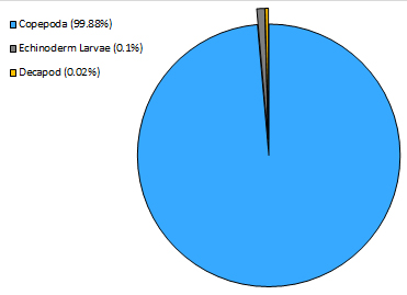
Figure 5. Composite figure which displays the depth profiles for Chlorophyll using the fluorescence data from CTD, Chlorophyll from water samples, Oxygen saturation from CTD, Oxygen from water samples, and PAR from CTD, where each graph represents each station (C30, C31, C32, C33, C34, C35, C36 and C37). Each graph also displays the 1% PAR depth line.

See how the Dissolved oxygen samples are processed in the laboratory by clicking on the picture!

Disclaimer: The views and opinions expressed are solely those of the contributors, they do not reflect the views and opinions of the University of Southampton.

Table 1. Table displaying the environmental conditions and times (UTC) of data collection offshore.

Table 2. Table showing the coordinates and time of sampling (UTC) at each station (30-37) offshore.

C30

C31

C32

C33

C34

C35

C36

C37

A

B

A

B

A

B

CTD

Salinity

Figure 10A displays many salinity spikes with increasing depth seen at all stations, however this is due to the error from the CTD and does not truly represent the variation in salinity at the stations. In general a trend can be deducted that the salinity is fairly homogenous for all stations, where the line for each station overlap considerably. There is a slight increase in salinity of approximately 0.1 with depth for all stations, for example for station C34 at depth 1.8m, salinity of 35.26, where at 58.8m has salinity of 35.34. This is due to the higher salinity and cooler temperatures (seen in Fig.10B), leading to the lower density water which sinks below the less dense water. The stations closest to the shore are also seen to have lower salinities at all depth than stations further from the shore (i.e. C31 and C32), for example at 20.5m depth station C37, there is a salinity of 35.3, whereas at station C32 there is salinity of 35.4. This is likely due to the input of freshwater from rivers which has greater influence closest to the shore.  

Temperature

The surface temperature ranged from 15.5-17.5oC across all station where the stations closest to the shore (Stations C37, C36, C35 and C30) had surface temperatures at the lower end of the range, and the stations with increasing distance from the shore (Stations C34, C33, C31 and C32) displayed corresponding larger surface temperatures. The sea temperature at the surface is greater than at depths due to the solar heating effect that occurs resulting from greater sunlight in the spring season. Therefore the figure displays a clear front that occurred with decreasing distance from the shore, occurring between the distance from shore for station C30 and C34, where there is a change in properties due to the becoming well mixed, over a relatively short distance. Stations C37, C36, C36 and C30 display a more homogenous mixed water column; where even at greatest depth 46m (for station C35) the temperature remained within the range 14.0-16.2oC due to the increased mixing resulting in the reduced thermocline. Whereas for the stations C34, C33, C32 and C31, at depth of 8m the temperature has a sudden decrease, indicating a strong thermocline, to reach temperature as low as 12.8oC at 66.8m depth. This thermocline is therefore more prominent is stations C32 and C31 which are further from the shore due to the reduced tidal input.

Turbidity

At the surface the stations closest to the shore have greater turbidity than stations furthest from the shores; for example at depth 5m at station C32 has a turbidity of 0.213 NTU, whereas at station C37 there is a turbidity of 0.240 NTU. This trend continues throughout the depth of the water column. The increasing turbidity with reducing distance from the coastline is likely related to the increase in phytoplankton resulting from the increasing nutrient supply from riverine input, as well as organic detritus, and related to the resuspended erosion sediments occurring due to shoreline erosion. There is noticeably increasing variation in turbidity with increasing depth after the thermocline of 20m. Markedly, at the base of each depth profile for each station there tends to be a slight increase in turbidity, this could be related to the resuspension of sediments due to the tidal friction from currents within the lowest few meters near the seabed. The high turbidity at the surface waters of station C34 is likely caused by the turbulence from propellers of the RV Callista. The most prominent increase in turbidity is seen at station C34. This station was sampled at 13:15 UTC, which occurred directly after low tide at 12:21 UTC. This increasing turbidity with depth at the station therefore is caused by the flooding tide, which resulted in resuspension of the benthic sediments.

Fluorescence

The fluorescence varied considerably with depth. It indicates chlorophyll concentrations and therefore the abundance of phytoplankton with depth. In general, at the surface waters (0-10m depth) and near the seabed (45-60m depth) the fluorescence remains relatively low and constant, where fluorescence ranged from 0.05-0. 10mg/m3 across all stations, whereas between the depths 20-40m the fluorescence increases to above 0.10mg/m3. This is where the chlorophyll maximum and phytoplankton blooms occur as a result of an increased supply of nutrients from below the thermocline, due to increased mixing (seen at 20m in Fig. 10B), and supply of sunlight is maintained within the euphotic zone.  Above this, in the depth 0-10m, this nutrient supply is limiting photosynthesis, whereas below 40m irradiance is limiting. However some phytoplankton copes in the nutrient limiting environment therefore the fluorescence is not at zero. The stations C31, C32, C33 and C34, display a significant increase in fluorescence, in particular C33 where at 31m depth reaches fluorescence of up to 0.28mg/m3. However stations C36 and C37 display less change in fluorescence throughout the depth of the water column as these stations are closer to the shore and therefore have a shallower depth.

Figure 10A. Salinity profile with depth for the water column at each of the 8 stations offshore of west of Falmouth, using the CTD on the RV Callista.

Figure 10B. Temperature profile with depth for the water column at each of the 8 stations offshore of west of Falmouth, using the CTD on the RV Callista.

Figure 10C. Turbidity profile with depth for the water column at each of the 8 stations offshore of the west of Falmouth, using the CTD on the RV Callista.

Figure 10D. Fluorescence profile with depth for the water column at each of the 8 stations offshore of the west of Falmouth, using the CTD on the RV Callista.

OFFSHORE

Falmouth 2017 - Group 7