GROUP 11
FALMOUTH 2017

Figure 3: Shows temperature decreases with depth for all stations, consistently highest at station 25.
From the Niskin bottles:
- Dissolved oxygen: Measured at 3 Bill Conway stations (Surface: 22, 23 & 24, mid depth 24). 1ml of manganese sulphate and 1ml of potassium iodide was added to bottle washed with sample and inverted to mix.
- Dissolved oxygen content was then determined using the Winkler method (Grasshoff et al. 1999)
- Chlorophyll: Measured at all 8 stations. 50ml filtered though filter paper, which is then submerged in acetone.
- Phosphate & Nitrate: Measured at all 8 stations. Filtered using a syringe into a brown bottle, ensuring no air bubbles.
- Silicon: Measured at all 8 stations. Sample filtered into plastic bottle using a syringe.
- Phytoplankton: Collected sample preserved in LUGOLS bottles. Phytoplankton were counted by eye using a microscope.
Estuary Spatial Series
Vessel: Bill Conway
Date: 07/07/17
Location: Start point - Port Pendennis Marina
Time: 08:30- 12:00 UTC
Weather: Initially 2/8 cloud cover, increased to 4/8 cloud cover with almost no wind
Sea state: Smooth with respect to the Douglas Sea Scale
Tide times: Low tide at 10:27 UTC, high tide at 16:17 UTC
Vessel: Winnie the Pooh
Date: 07/07/17
Location: Start point - The King Harry Pontoon (50º 12’ 58’’ N 005º 01’ 59.5’’ W)
Time: 12:0 0- 16:00 UTC
Weather: Initially 4/8 cloud cover, cleared to 2/8 cloud cover with almost no wind
Sea state: Smooth with respect to the Douglas Sea Scale
Tide times: Low tide at 10:27 UTC, high tide at 16:17 UTC (flood tide)

Observing nutrient profiles and properties, as well as chlorophyll levels and how they vary across a salinity transect. Conway was able to sample various depths throughout the water column at 4 locations, whilst Winnie the Pooh sampled at a constant depth (0.3m below the surface) at 4 locations. Using data from both vessels to create an estuarine mixing diagram.

Image shows 8 stations used to create a spatial series in the estuary. On Bill Conway (dark blue) depth profiles were taken at each station. On Winnie the Pooh (light blue) only surface samples were taken. Combining the data collected at all these stations enables the creation of a mixing diagram with a wide variety of salinity.
O
P
Q
25
24
23
22
N
Falmouth
Truro
On the Bill Conway:
- Using a CTD depth profiles were produced for fluorescence, temperature, salinity and transmission at 4 stations.
- Niskin bottles collected 2 water samples at each of the surface, mid and deep depths.
- ADCP transects were used to measure flow velocity and direction.
- A plankton net (mesh: 200μm, diameter: 0.5m) was towed for 5 minutes from station 22 to collect zooplankton.
On Winnie the Pooh:
- T/S probe was used to measure the temperature, salinity and pH of the water at 4 stations.
- A Niskin bottle collected surface water samples (0.3m) at each station to sample the surface water.
- A plankton net (mesh: 200 μm, diameter: 0.5m) was towed for 5 minutes to collect zooplankton samples.

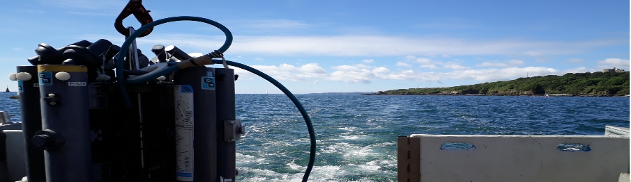
Image shows CTD profiler with Niskin bottles on Bill Conway

Figure 2 shows temperature decreased with depth for all stations. Surface temperature was lowest at station 22 (15.6ºC) and highest at station 25. Temperature at station 24 decreased from 16.5ºC at the surface to 15.25ºC between the surface and 12m then further decreased over the next 10m to around 14.6. Temperature at station 23 decreased from 16.0ºC at the surface to 14.5ºC at depth.
Figure 9 shows station 22 showed a drastic increase in nitrate concentration within the first few meters, starting at 1.2µmol/l at the surface and increasing to 6µmol/l before decreasing to a concentration of less than 1µmol/l at a depth of 30m. Station 23 showed the lowest nitrate concentration throughout the water column out of all four stations. It rained constant with depth with an average concentration of 0.5µmol/l. Station 24 nitrate concentration decreased from 5.5 to 4µmol/l at 5m. This then increased at 12m to 6.5µmol/l. Station 25 had a high surface nitrate concentration of 5.8µmol/l. The rate of decrease in nitrate concentration with depth increased after a depth of 5m.
Figure 10 shows Silicon concentrations for station 22 decreased from 0.75µmol/l to 0.25µmol/l within the first 4m of the water column. Subsequently it remains constant until a depth of 29m. This station also has the lowest silicon concentration out of all the stations. Silicon concentration at station 23,24 and 25 decreased with depth. For station 23, silicon concentrations dropped from 1.75µmol/l to 0.5umol/litre. Silicon concentrations for station 24 dropped from 2.25µmol/l to 1.0µmol/l and 3.5µmol/litre to 1.25µmol/l for station 25. Station 25 has the greatest range in silicon concentration from surface to depth.
Figure 11 shows station 22 has a phosphate surface concentration of 0.3µmol/l and a 30m depth concentration of 0.39µmol/l. Within the first 5 m, the concentration of phosphate decreased to 0.13µmol/l before increasing again with depth. Similarly, station 24 follows a similar trend, with it’s initial surface value at 0.57µmol/l before decreasing in the first 6m to 0.28µmol/l before increasing again to 0.49µmol/l at a depth of 8m. Station 23 is the only station to increase consistently with no decreases in concentration. With a steady increase of it’s surface value of 0.12µmol/l to 0.4µmol at 10m, remaining steady between 10m and 28m at a concentration of 0.41µmol/l.
Station 25 shows an initial increase in phosphate concentrate with depth from 0.35µmol/l at the surface to 0.52umol/l at 8m before decreasing to 0.4µmol/l at 18m.
Fluorescence (shown in figure 1) is lowest at the surface for station 22 and 23 (~0.175), increasing and fluctuating around 0.25 with increasing depth. Stations 24 and 25 were higher at the surface (0.25), increasing to about 0.35 around 5-10m, and then decreasing to around 0.225 at 12m.
The transmission is highest for station 23. At the surface at 4.71 transmission value then it decreases rapidly in the first 3m down to 4.63. then it increases as depth increases down to 27m to 4.73 then at that depth it decreases rapidly down to 4.69.
Station 22 has the second highest transmission down to around 10m after which it has the lowest transmission values of all the stations. Its transmission value remains the most constant with depth in comparison to other stations, except for a few small fluctuations (4.66 T-value).
Station 24 has the second lowest transmission of all the stations, and increases with depth from T-value of 5.59 to 4.65.
Station 25 has the lowest transmission of all the stations until a depth of around 8m and then it increases to one of the highest values of 4.73 at around 12m before rapidly decreasing down to 4.65.
Figure 3 shows the salinity of Station 22 remained constant throughout the water column to a depth of 30m. At the surface the salinity was about 33.75 and at 30m the salinity was 33.85. After a depth of around 10m it had the lowest salinity of all the stations. Salinity at station 23 was higher than the other stations throughout the water column. The salinity for this station stayed around 34.25. Within the first 10m of the water column the salinity increased gradually with depth, in contrast to the bottom half of the water column where salinity decreased slightly with depth. Station 24 had a salinity of 33.6 at the surface which increased gradually to a salinity of 33.8 at 10m. Station 25 had the lowest salinity at the surface, a value of 32.4. With an increase in depth, salinity significantly increased to a value of 33.9.

Figure 1: Shows fluorescence fluctuating for all stations, and peaking nearer the surface at stations 24 and 25.

Figure 4: Shows turbidity remains relatively constant with depth at station 22, while increasing with depth at stations 23, 24 and 25

Figure 2: Shows salinity is relatively constant with depth for stations 22, 23 & 24, but increases with depth at station 25.
CTD Profiles
ADCP Transects
Richardsons


Nutrient Profiles


Figure 5: ADCP transect including station 22
Figure 6: ADCP transect including station 23
Figure 7: ADCP transect including station 24
Station 22 (Figure 5) was the lower estuary closest to the mouth of the estuary and open water, sampled at around 8:40 UTC. Generally, for station 22 there is higher velocity magnitude towards the mouth of the estuary as a posed to approaching the upper estuary. This is likely due to the tidal effect being greater than the riverine near the mouth of the estuary. Also, there is higher velocity magnitude towards the surface layer, hence near the mouth of the estuary there is greater velocity on the surface layers, probably because of wind at the mouth of the estuary as it is more exposed than the upper estuary.
In general, station 23 (figure 6), which was further up the estuary than station 22, sampled at around 10:15 UTC. There was a uniform spread of low velocity at all depths. This could be explained by the sampling been done before low tide at 10:27 UTC, which meant that a lot of the water was not being moved, hence there was not much mixing.
For station 24 (figure 7), which is furthest up the estuary, sampled around 10:58 UTC. The velocity is higher at depth here, this is after the low tide so there is more mixing from the flood and so higher velocity is observed at depth and mixing as it is between low tide and high tide, hence tidal mixing is stronger on the flood tide (Simpson et al., 1990).

The Richardson number was calculated using the following equation:
This took into
account the acceleration due to gravity, overall density within the water column
and change in depth and salinity from point to point. There is a simplified equation
which doesn’t take into account shear components, this only occurred where there
were flows in opposing directions and a difference of ~45o.
The Richardson number
gives an idea of the stratification of the water column, 0.25 < Ri would relate to
a stable column and Ri < 0.25 would indicate shear velocity mixing in the water.
Data was smoothed by sampling every 3 depths to remove fluctuations. For the estuary
it can be seen that there is a general trend of lower Ri number towards the surface
with a slight increase to depths between 10-20metres and a following decline. The
largest variance in Ri occurs the further southwards, and closest to the open ocean.
Station 22 was the only location to exhibit a value over 1, (~2). When a value exceeds
1 it is said to have reached critical value, this would indicate that stratification
within the water column is likely. A value below 0.25 indicates that mixing is likely
to occur, any value in between these two is a transition zone. The two stations to
indicate this transition zone are station 22 and 25, both at a very similar depth
of ~11 metres. Stations 23 and 24 remain below the critical value of 0.25 with values
staying between 0.1-0.001, indicating that mixing is likely. Large fluctuations can
be seen in the majority of data, sometimes varying by a factor of 2 to the next depth,
station 23 sees the least variance suggesting it is the most consistent and ‘stable’
water column.
Figure 8: The estuary shows a general trend towards mixing being likely within the water body as a whole, with a potential transition to stratification in Station 23 and Station 22 exceeding the critical value of 1 indicating stratification being likely to a small degree.
Phsysical
From the results we can see a shear driven system, one in which buoyancy may not be important. This may not be what is expected from an estuary due to the high input of fresh water to the system with cooler submarine groundwater discharge being a significant input for freshwater flow. This water would enter the system at a lower temperature and a lower salinity than the water it would be mixing with, resulting in differences between buoyancy. September generally sees the highest SSTs and thus a higher level of stratification, the ocean takes a while to transfer heat and a lag time from heating exists. Therefore, a high percentage of mixing is indicative a more uniform body of water. A further complication was the tide at the time, the flooding tide would have led to increase shear between the water and estuary seabed, showing a more well mixed water body at the time. However, a study by Polzin (1995) indicated that dissipation rates of well mixed bodies can take past the critical value of 1.00 < Ri but still associated with it. So the peak at ~18m may not be a change from turbulent flow to laminar flow. It may also relate to an error in the calculation step or bad measurements from on-board equipment.


Estuarine Mixing Diagrams
Figure 12 displays an inverse relationship between nitrate concentration and salinity. The lowest salinity sampled had a salinity of 20, which had a nitrate concentration of ~115µmol/l, whilst the highest salinities observed were ~35 with corresponding nitrate concentrations of less than 20µmol/l.
It is also observed that nitrate behaves non-conservatively as the data points lie below the theoretical dilution line, indicating the removal of nitrate. The removal of nitrate could indicate uptake by phytoplankton for important biological processes. Another possible reason could be nitrification. Nitrification is the oxidation of ammonium to nitrate, a process which is sensitive to changes in salinity. As the water changes from fresh river water to saline sea water, the rate of nitrification lowers and the level of nitrate available decreases. (Giblin, 2010)
The lowest salinity was observed to be ~0 with a phosphate concentration of ~1.6µmol/l. The highest salinity observed was ~38 with a phosphate concentration of 0.3µmol/l. The lowest phosphate concentration was 0.0µmol/l at a salinity of ~34. The highest phosphate concentration was 2.8 µmol/l with a salinity of 25.
Figure 3 indicates non-conservative behaviour for phosphate with data points lying above the theoretical dilution line, suggesting addition of phosphate into the estuary. An increase in phosphate concentrations may be attributed to the fact that the area surveyed was in close proximity to sewage outfall. This may cause a change in pH which would result in the desorption of phosphate into the solution. (Smith & Longmore, 1980). Due to human error, Group 11’s phosphate data was unable to be analysed and so Group 10’s have been used as substitute. The lowest observed phosphate concentration value is likely to be anomolous due it being the only value below the TDL as well as showing a reading of 0.
It is observed in figure 13 that there is an inverse relationship between silicate concentration and salinity. As the salinity increases, silicate concentration decreases. The lowest salinity observed was to be 20 with a silicate concentration of ~21µmol/l, whilst the highest salinity concentration recorded was ~36 with a silicate concentration of ~1 µmol/l, also being the lowest silicate concentration recorded.
Non-conservative behaviour is also demonstrated here as the data points lie below the theoretical dilution line suggesting the removal of silicate from the estuary. This removal of silicate could indicate biological uptake, specifically by diatoms for the formation of their frustules (Gross, 2012). This removal could also be attributed to adsorption and flocculation of silicate from the water column into the sediment.
Figure 12 shows an estuarine mixing diagram for nitrate concentration against salinity for River Allen and the Fal Estuary. A theoretical dilution line (TDL) was included between the river endmember and sea endmember.
Figure 13 shows an estuarine mixing diagram for silicate concentration against salinity for River Allen and the Fal estuary. A theoretical dilution line was included between the river endmember and sea endmember.
Figure 14 shows an estuarine mixing diagram for phosphate concentration against salinity for River Allen and the Fal estuary. A theoretical dilution line was included between the river endmember and sea endmember.
Figure 9: Nitrate Profile with depth
Figure 10: Silicate Profile with depth
Figure 11: Phosphate Profile with depth


Figure 15:P ie chart showing the abundance of phytoplankton species found per 1ml water sample. Counted under a light microscope, for station 22.
Figure 16: Pie chart showing the abundance of phytoplankton species found per 1ml water sample. Counted under a light microscope, for station 24.
Figure 17: Pie chart showing the abundance of phytoplankton species found per 1ml water sample. Counted under a light microscope, for station 25.

Figure 1 shows that a total of 294 individuals were counted which is equivalent to 294,000 cells/l. The most abundant species present appears to be Dinoflagellates, making up 66% of the total counted (195000 cells/l). The second most abundant species present appear to be Psuedo-nitzschia making up 30% of the total count (89000 cells/l). All 7 other phytoplankton counted accumulate to only 4% of the total counted.
Figure 2 shows that a total of 53 individuals were counted which is equivalent to 53,000 cells/l. This station unlike Station 22 has abundances of phytoplankton with similar percentages to each other. The most abundant species present appears to be Cylindrotheca spp. making up about 36% of the total count (19,000 cells/l) this is significantly more than at station 22 where less than 1% of the phytoplankton counted were Cylindrotheca. The second most abundant species appears to be Proboscia truncate making up about 23% of the total count (12000 cells/l).
Figure 3 shows that a total of 17 individuals were counted which is equivalent to 17,000 cells/l. The most abundant species here appears to be Nitzschia spp. making up about 59% of the total count (10000 cell/l). The second most abundant species appears to be Chaetoceros making up about 29% of the total count (5,000 cells/l).
Figure 4 shows that a total of 630 individuals were counted which is equivalent to 1206 per m3. The most abundant species appears to be Copepoda making up about 61% of the total count (731 per m3). The second most abundant species is observed to be Echinoderm larvae accounting for over 25% of the total amount of species observed.
Figure 18: Pie chart showing the abundance of zooplankton species found per 10ml water sample. Counted under a light microscope, for station 22.
The water column structure of the estuary measured by Conway is as expected, wherein, the salinity decreases away from the mouth of the estuary, with the exception of station 22, the salinity is lower than expected for a station that is closest to the mouth of the estuary; this could be due to the riverine input that is located next to station 22 providing fresher water.
Stations 22, 23 and 24 display little variation in salinity with depth which indicates that they are well mixed. These stations are closer to the mouth of the estuary and therefore are exposed to winds, storms and a large seawater input, hence mixing is encouraged.
Station 25 is the furthest from the mouth of the estuary and therefore has the lowest salinity as it is closest to the fresh water input from the river. Fresh water is less saline and therefore less dense compared to sea water. The fresh water input remains at the surface overlying the more saline estuarine water. This indicates that the head of the estuary is not well mixed in comparison to stations 22 and 23 nearer the mouth. This shows that the riverine input dominates tidal currents.
Due to the relative shallowness of estuaries great ranges in temperature can be observed, for instance, stations 22 and 23 were sampled to a depth of ~28m, in comparison stations 24 and 25 could only be sampled down to a depth of 12m. In relation to temperature changes, there was a decrease in surface temperature as you move towards the mouth of the estuary. Station 22 has a surface temperature of ~15.5C° and a thermocline at 6m, indicating a stratified water column. Stations 23 and 24 show a similar stratification to station 22. On the other hand, station 25 has the highest surface temperature of 17.5C° but is less stratified than previous stations.
As depth increases, initially the speed of sound will decrease because of temperature decreasing but at a point, the temperature is more constant which is seen after 10m for all 4 stations. The speed of sound will then begin to increase again with depth and pressure. (Flatte et al, 1979)
Chemical
During spring and summer, phytoplankton blooms occur which consume nutrients such as nitrate for biological processes. This explains the decrease in nitrate concentration with depth across stations 22, 23 and 25. Station 24 doesn't follow this trend and this could be due to nitrate riverine inputs. This could also be attributed to the sewage outfall located in close proximity to station 24. Bacteria oxidise ammonia to nitrite which is then converted to nitrate, thus increasing the concentration. This could also be an explanation to the increase in phosphate concentrations, in an area that a decrease would be expected as chlorophyll increases.
The two stations upstream, stations 24 and 25, showed higher concentrations of chlorophyll in the surface than the two station downstream. This could be a result of high nutrient input from the river which would indicate high phytoplankton numbers, resulting in high fluorescence values.
Biology
Copepods are mainly distributed near the seabed during the day and towards the surface waters at night, as well as this most are found above salinities of 27. So mostly near the outer estuary which is where the Conway sample stations were situated. (Cailleauda et al., 2007)
Due to human error, the plankton abundance data is unlikely to be accurate due to
inexperienced counting increasing the risk of a misidentified species being consistently
misidentified causing incorrect and inconsistent counting. Furthermore, having 5
different people counting means increased chances of inconsistent counting methods
and identification.
The dominant phytoplankton species at station 22 were dinoflagellates
but pseudo-nitzchia were still a very large proportion.
The dominant phytoplankton
species at station 24 were cylindrotheca spp.
The dominant phytoplankton species at
station 25 were pseudo- nitzchia.
The dominant zooplankton species at station 22
were Copepoda.
| Meet the Team |
| Time Series |
| Spatial Series |