Falmouth 2016 Group 9
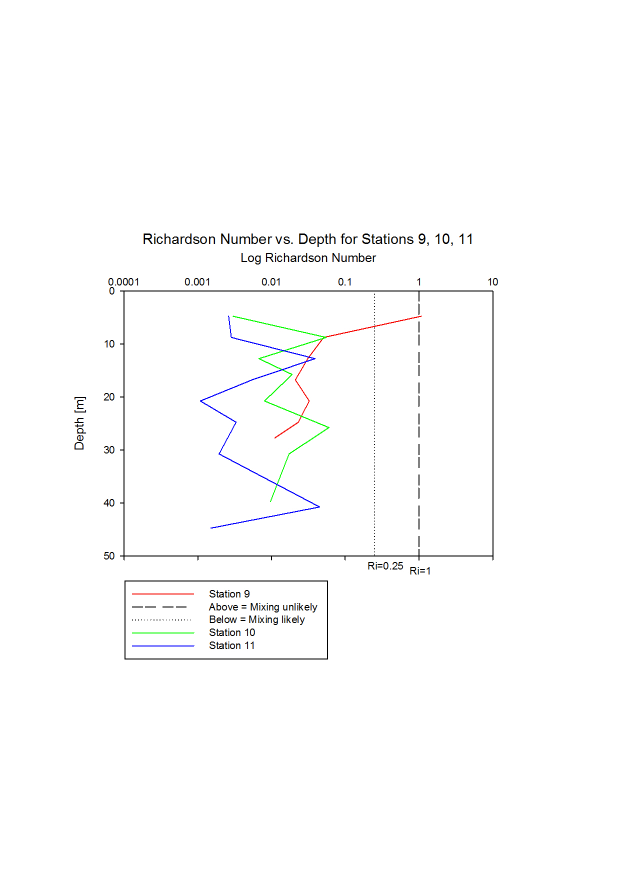
The Richardson numbers calculated from the offshore ADCP data are relatively low. These low values (below 0.25) indicate that small scale turbulence is likely to develop, leading to mixing in the water column (Linacre & Geerts, 2006). The only station where a number greater than 1 is produced is at the surface of station 9. This is the station closest to the outflow of the estuary so could have surface influence from less dense freshwater, flowing on top of the seawater. The density difference created by this will result in more laminar flow, hindering mixing. Overall, small scale turbulent mixing is indicated throughout the water columns of all stations.
Linacre, E., & Geerts, B. (2006). The Reynolds', Richardson's, and Froude numbers.
Retrieved from UW Atmospheric Science: www-
Contents:
Physical:
A. Salinity Profiles
B. Temperature Profile
C.
Transmission Profiles
D. PAR Profiles
E. Flourometery Profiles
F.
Full Physical Data by Station
Chemical:
G. Dissolved Oxygen Profiles
H. Nitrate Profiles
I.
Phosphorus Profiles
J. Silicon Profiles
Biological:
K. Chlorophyll Profiles
L. Zooplankton Profiles
Metadata:
|
Station |
Time (UTC) |
Location |
|
9 |
08:36 |
Lat: 50˚ 07 472 N Long: 004˚ 58 921 W |
|
10 |
10:29 |
Lat: 50˚ 05 685 N Long: 004˚ 52 029 W |
|
11 |
13:04 |
Lat: 50˚ 06 725 N Long: 004˚ 42 822 W |
|
12 |
14:45 |
Lat: 50˚ 02 986 N Long: 004˚ 44 042 W |
Physical Results:
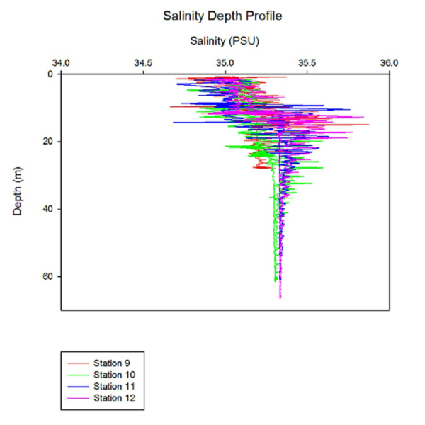
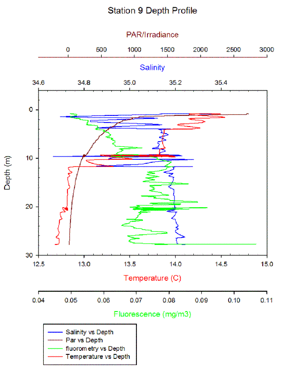
The surface levels of the salinity range from approximately 34.8-
The lower salinity at surface waters may be due to coastal fresh waters from the estuary, especially effecting station 9 due to the proximity of the coastal waters. The deep water results of a slightly higher salinity may be due to the open ocean waters of saltier, denser water sinking to lower depths.
The large amount of spikes that occur in the data are due to a delay within the CTD of the temperature and conductivity sensor, which are used to calculate the salinity.
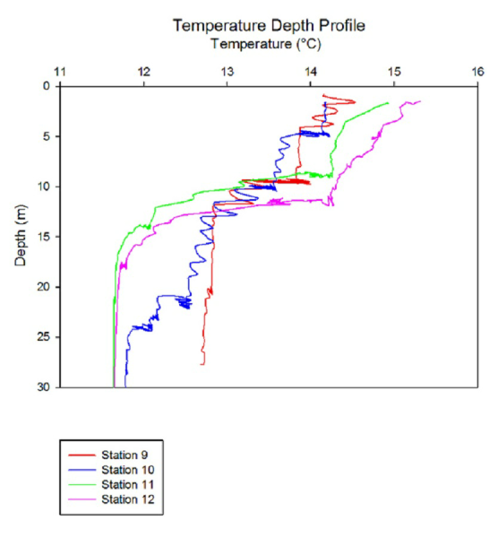
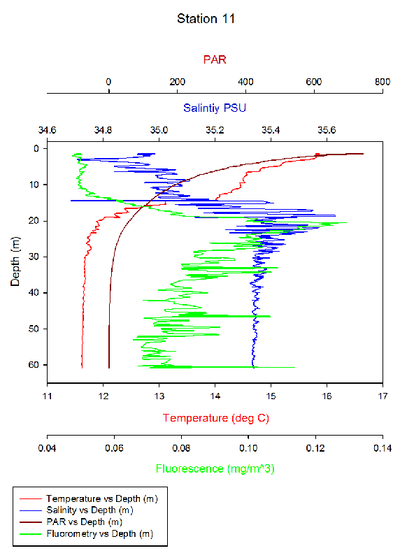
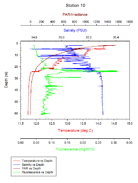
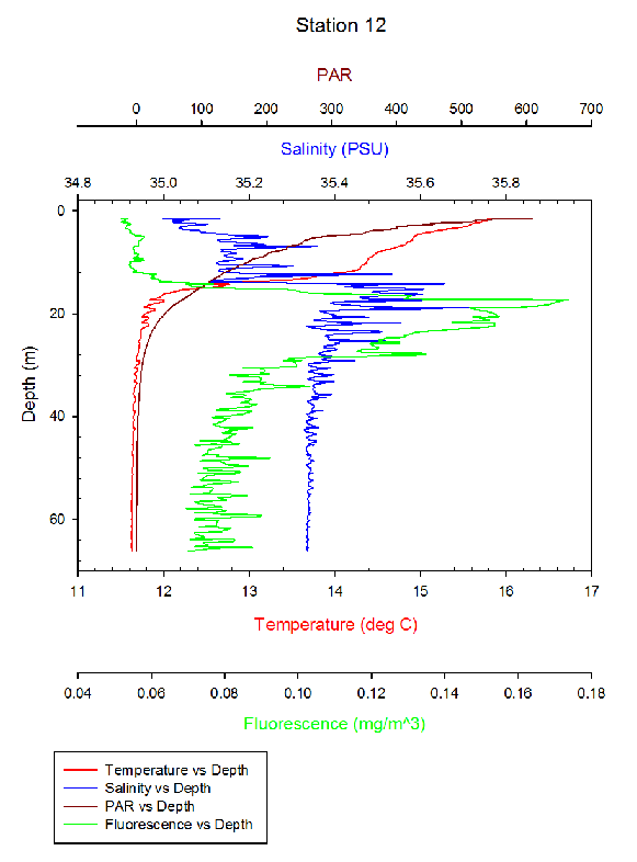
The temperature profiles of each of the 4 stations display variations in the thermal structure of the water column at each location. When the CTD was lowered through the water column at station 9, an unusual signal was seen on the depth profile. This is seen as horizontal variations on the graph, which theoretically should not be seen. Dr Boxall concluded that there was a problem with the pump on the CTD when sampling this station. Ignoring this horizontal variation, a gradual decrease in temperature with depth is observed until around 10m depth, where the thermocline is observed. Here a rapid decrease in temperature with depth occurs, and after around 12/13m, temperature is fairly uniform with depth at approximately 12.7°C. Station 10 shows a series of smaller thermoclines at 5m, 10m, and 21m before uniformity is seen below 25m. The deep water temperature at station 10 is comparatively lower than at station 9, despite the fact that surface temperatures were the same. Station 11 has a much simpler profile, beginning at a greater surface temperature of nearly 15°C, with a thermocline starting at 10m, becoming uniform with depth below 15m. Station 12 has a slightly higher surface temperature, and a slightly lower (13m) thermocline. Temperatures are uniform with depth below 17m at about 11.6°C.
The general trend is that the degree of thermal stratification increases with distance offshore (i.e. 9, 10, 11/12 respectively). This is due to reduced influence from tidal mixing with distance from the coast. Station 9 will experience the most tidal mixing, reducing stratification. Greater tidal mixing at this station is also a possible explanation for the comparatively greater bottom water temperatures seen here. Stations 11/12 are very similar distances offshore and so experience similar levels of stratification. Initial stratification will have begun in spring, and will increase throughout the summer. This occurs due to increased irradiance, warming the surface layers of the ocean, promoting water column stability due to less dense water overlying more dense water.
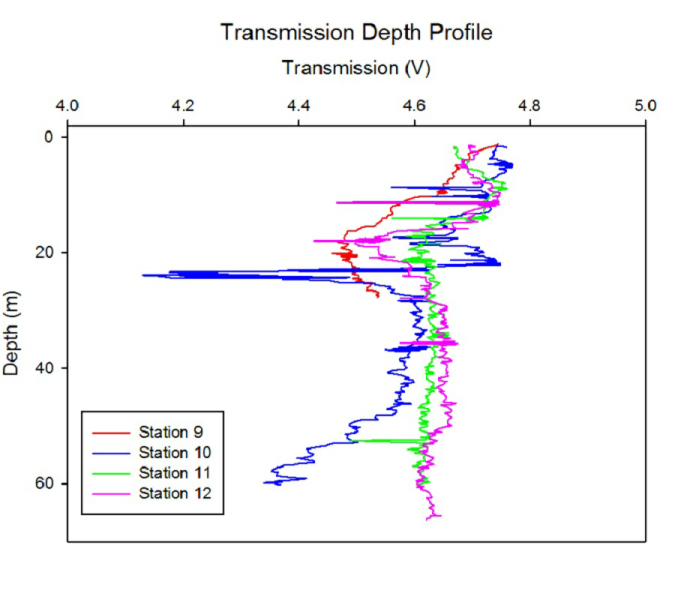
Transmission is used as an indication of turbidity within the water column; with the lowest values showing the highest amount of turbidity. It is measured by light attenuation in the transmissometer so will be affected by suspended particle matter as well.
It would be expected that the transmission values should be lower at the surface
due to wind stresses creating more turbulence. However our results show that in surface
waters the turbidity is very low in surface water (between 4.65-
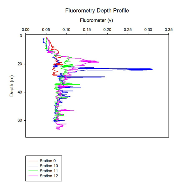
One of the most significant changes in the transmission graph is in station 10, where the transmission values drop significantly from 4.7 to 4.1 v at a depth of approximately 24 metres. This corresponds with the large fluorescence peak at Station 10, which suggests that a large patch of phytoplankton may be found here and reducing the amount of light attenuation within the transmissometer.
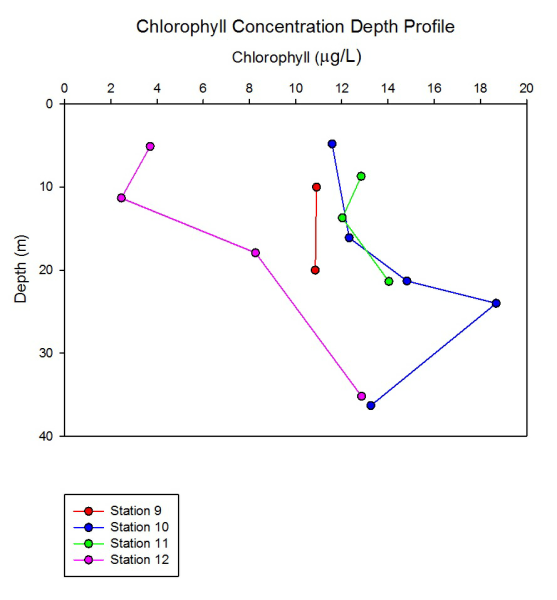
Fluorescence readings relate to the fluorescent nature of chlorophyll; the main molecule affecting the fluorometer readings. In all 4 stations, fluorescence increases gradually with depth for the first 20m. Station 9 reaches its maximum at around 30m. Station 10 has a very large chlorophyll maximum at around 23m depth. The maximum fluorescence reading for station 10 is about 0.32v, almost double the value of station 12’s maximum (the station with the second largest reading). Once the maximum is reached, fluorescence appears to decrease very gradually with depth for all stations. There are some significant fluctuations, which most notably occur with stations 10 and 12.
It appears that the stations see chlorophyll maximums at around 20m. These chlorophyll maximums relate to concentrations of phytoplankton populations. Phytoplankton tend to accumulate around the pycnocline in stratified waters, so that they can utilise nutrient rich waters below and maintain their position in the euphotic zone. The chlorophyll maximums occurred at similar depths/just below the haloclines shown in the salinity plots, and just below the thermocline depths shown in the temperature plots. Here the water column is mixed, allowing for improved distribution of nutrients.
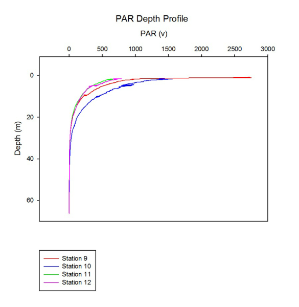
The irradiance within the water shows an exponential decrease as the depth of water increases. The surface irradiance values were lower in Station 11 and 12 (approximately 673v and 780v respectively) compared to Station 9 which was measured at the beginning of the day which had a measurement of 2740v in surface waters. This is due to the fact that as the day progressed, the weather conditions worsened, with Station 11 and 12 measured under cloudy and misty conditions, reducing the amount of solar radiation and reducing the amount of irradiance in surface waters.
Station 10 has a lower attenuation rate compared to the other stations, which could
suggest a larger phytoplankton bloom, as a higher amount of light penetrates deeper
depths. This can be seen on station 10 profile, where there is a large phytoplankton
bloom between 20-
Below is a table of attenuation coefficients calculated by using our Secchi Disk measurements from each station using the equation: Light attenuation (k) = 1.46/ Secchi Disk (m) (Holmes, 1970).
Click to Enlarge.
Click to Enlarge.
These coefficients do generally agree with the CTD data; Station 10 does have a significantly lower attenuation coefficient and suggests that the other stations have similar attenuation coefficients. An approximation of the euphotic data can be taken by multiplying the Secchi Disk by 3, but this is a rather rudimental approximation due to inaccuracies when using the Secchi Disk.
Reference:
Holmes, R.W. (1970) ‘The secchi disc in turbid coastal waters’ Liminology and Oceanography,
15 688-
|
Station |
Secci Depth (m) |
Light Attenuation (k) |
Euphotic Zone Depth Approximation (m) |
|
9 |
9 |
0.1622 |
27 |
|
10 |
12.7 |
0.115 |
38.1 |
|
11 |
9.1 |
0.1604 |
27.3 |
|
12 |
10.45 |
0.1397 |
31.35 |
Click to Enlarge.
Click to Enlarge.
Click to Enlarge.
Physical data was attained using 3 pieces of equipment: A CTD rosette featuring niskin bottles, an ADCP and a secchi disk. Time, location and maximum depth were recorded on arrival at each station. Once ready, the deck crew deployed the CTD, following instructions from those working at the computer. One person was positioned to relay messages between the computer operators and the deck crew/winch man. On descent, the CTD transferred live data to the computers and this immediately began constructing depth profiles. Just prior to maximum depth being reached, analysis of the depth profiles was made in order to decide on what depths to fire the niskin bottles used to collect water samples for chemical analysis. This included identification of the thermocline as well as the chlorophyll maximum from the fluorescence data. The CTD continued to recorded data on ascent which allowed for further checking and confirmation of depth profiles. The CTD was then brought back on to the ship where chemical analysis began, collecting and analysing the samples from the niskin bottles.
The CTD recorded various physical parameters including salinity, temperature, turbidity, irradiance and density. The ADCP was utilised to observe backscatter variations with depth, as well as calculations of the Richardson number to allow for an understanding of mixing in the water column. A secchi disk was used to obtain the secchi depth for further information on irradiance. The same person took this measurement every time in order to prevent perception differences due to eye sight.
The Richardson number (Ri) is a dimensionless number which allows characterisation of flow types (laminar or turbulent) within the water column. It is defined as the ratio between the buoyancy term and the flow gradient term (Turner, 1980).
N = Buoyancy Frequency – a measure of stratification
du/dz = Vertical gradient of horizontal velocity (change in velocity/change in depth)
Richardson numbers of less than 0.25 mean that the flow is likely to develop small scale turbulence. Richardson numbers of greater than 1 mean that small scale turbulence is unlikely to develop, and the flow is said to be laminar. By using calculated Richardson numbers for different depths in conjunction with CTD data, layers of stratified features such as thermoclines and tidal mixing fronts can be identified.
*** When the CTD was first deployed at station 9, the descending depth profile recorded an unusual signal, featuring unusual horizontal fluctuations of the temperature readings in the depth profiles. Dr Boxall concluded that this was a problem with the pumps on the CTD. This problem appeared to have cleared by the next station, but may be responsible for some unusual variation in the station 9 temperature data.
Lab methodology:
To produce 3 replicate samples per depth, 3 50ml samples were taken at each depth
and filtered using a GFF. The filter papers from these were placed into plastic test
tubes and submerged in 6ml of acetone to ensure preservation until laboratory analysis.
Chlorophyll concentrations were determined by obtaining absorbance readings from
a 10-
Dissolved oxygen samples were the first samples collected from the niskin bottles. The samples were transferred to rinsed glass bottles, and the number of the bottle was noted. After collection, samples had 1ml of manganese sulphate and 1ml of alkaline solution added to each. This addition resulted in the formation of a precipitate, and the bottles were sealed and stored in a bucket of water to prevent exchange with the atmosphere. Laboratory analysis involved the use of an automatic titration system. The process began with pipetting 1ml of sulfuric acid to the glass bottle before a magnetic stirrer was used to completely break up the precipitate. The solution was then titrated with sodium thiosulfate. The total volume of sodium thiosulfate used in the titration and the weight of the bottle were used to determine the concentration of dissolved oxygen in the samples.
Nitrate and phosphate samples were filtered and placed in glass bottles. Silicon samples were filtered and placed in plastic bottles. After bringing our previously filtered samples of nitrate into the lab, we then filtered them again before beginning to process each sample. With these newly filtered samples, we injected the nitrate into a Flow Injection Analysis System in order to convert nitrate into nitrite. We were then able to use nitrite to obtain a nitrite/nitrate concentration result which was recorded on a tracer, drawing red and blue peaks. Using the standardised peaks, we could compare our sample trace to attain a concentration in µmol/L through the use of a calibration curve.
For each of the 14 phosphate samples 30ml was measured and 3ml of the mixed reducing reagent, containing ammonium molybdate, sulphuric acid, ascorbicacid and potassium antimony tartrate solutions, was also added. Further to this, one out of every 5 samples prepared was replicated to ensure accuracy. After roughly 30 minutes, the absorbance was measured by inserting the solution into a 10cm cell using the Hitachi U1500 spectrometer. Using the equation produced from the standards and blanks the phosphate average absorbance could be converted into concentration ( mmol/l).
15ml was taken from each of our samples to be mixed with 6 ml of Ammonium Molybdate,
then further mixed with 9ml of a Mixed Reducing Reagent. This reagent contained MQ
water, metal-
For phytoplankton, 100ml of unfiltered seawater was transferred directly to a glass bottle containing a lugol in order to preserve the phytoplankton for later laboratory analysis.
Zooplankton
A net was used for collection featuring 200μm mesh and 50cm diameter, and was lowered across the chlorophyll maxima (identified with the CTD depth profiles). On recovery, the net was rinsed with the hose and the zooplankton sample was transferred to a 100ml bottle. The sample was preserved with 100ml of 10% formalin solution to allow for later laboratory analysis.
Bibliography
Turner, J. (1980). Small-
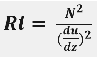

Station 9 showed a slight increase in dissolved oxygen concentration from 92% to just under 98% over a depth of 10 metres. Station 10 showed a general decrease in dissolved O2, starting at a concentration of 102% at the surface, down to 88% at 35m and with a small increase between 15 and 20m. At station 11, the graph shows a slight variation in dissolved O2, with a slight increase in the first few metres starting at 99.5% before a relatively steep decrease down to 96% at 20m. Station 12 follows a similar pattern to the previous station, with a starting measurement of 96% and increasing for the first few metres to 100% before a decrease in dissolved oxygen concentration down to 91.5% at 35m. The general decrease in oxygen at the majority of the stations is due to the reducing light levels with depth; this means there is reduced amounts of photosynthesis and therefore very little oxygen production. The highest levels of dissolved oxygen concentration should coincide with the phytoplankton blooms – where the amounts of oxygen production are high due to the levels of photosynthesis taking place.
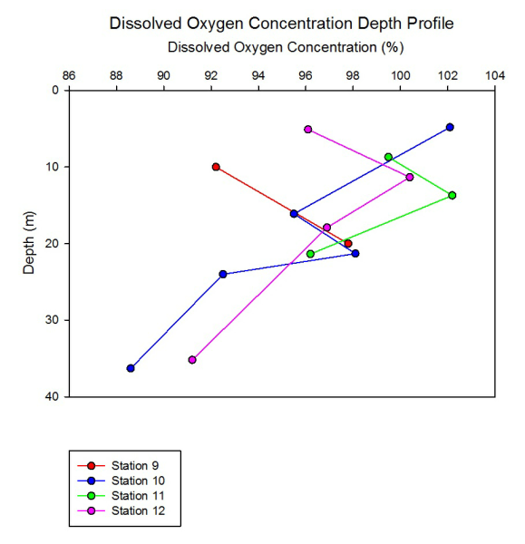
Nitrate concentrations showed far more variability than other nutrients at all stations
other than station 9 which appears to only be increasing in concentration with depth,
but might show more variability if more measurements were taken. Surface concentrations
varied with each station, with a low of 0.15µmol/L at station 10 and a high of 1.25µmol/L
at station 12. The highest level of nitrate concentration was measured to be 1.6µmol/L
at a depth of 25m at station 12, but in the graph, we may have seen station 9 see
a maximum somewhere just below 20m with more measurements. The variability in Nitrate
is due to the stripping of the nutrient at the surface by phytoplankton, similarly
to phosphate, since the upper layers of the water column have ideal conditions for
phytoplankton growth, hence the blooming. At depth, the lack of light makes the conditions
for primary production less ideal and therefore the concentrations of nitrate increase
with depth (Garside, 1985).
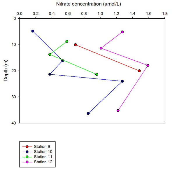
Concentration of phosphate increases with depth at all stations, with only slight variability being seen at station 10 which does fluctuate slightly. We took measurements down to 36m for stations 10 and 12 allowing sensible comparison at these depths; station 12 saw a much higher concentration in phosphate of almost 0.6µmol/L whereas station 10 was only recording a value of just over 0.2µmol/L. Phosphate is another element used by microorganisms such as phytoplankton in the form of phosphate at the surface levels, hence the minimum concentrations for each station being in the surface layers. At depth, the lack of light means phosphate is not removed from the water column.
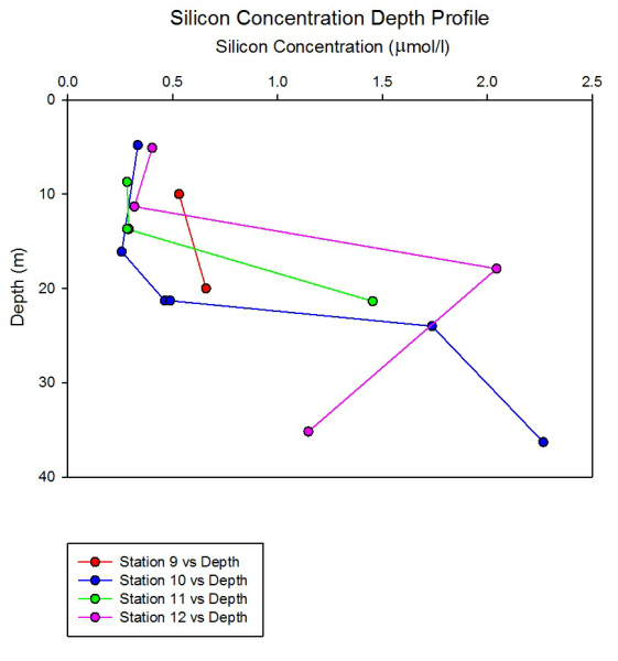
A general trend of increasing silicon concentration with depth can be seen at all stations except station 12 where a decrease from 2.0 to 1.1µmol/L can be seen in the graph. All stations appear to start at the same silicon concentration level at the surface of approximately 0.4µmol/L. Station 10 saw the largest value of concentration of 2.3µmol/L at a depth of 36m. Although very small traces of silicon are needed by organisms, it is an essential element in biology (Nielsen, Forrest H., 1984). The lower concentrations of silicon at the surface is due to the uptake and use of silicon by diatoms and radiolaria for making frustules out of silica. The higher levels of silicon are seen to be below the blooms of phytoplankton since, when they die, these organisms sink and hence silicon is returned to the water column.
Ref Nielsen, Forrest H.; Ultratrace Elements in Nutrition; Annual Review of Nutrition; 1984
Arrigo, K.R.; Marine microorganisms and global nutrient cycles; Nature Vol. 437; 2005
Click to Enlarge.
Click to Enlarge.
Click to Enlarge.
Click to Enlarge.
Introduction:
Coastal fronts are key features of coastal waters. Their presence and
structure is indicated by thermal stratification of the water column, which ultimately
influences nutrient distribution. The presence and structure of these fronts vary
with the seasons. Spring blooms of phytoplankton occur at the surface around these
fronts, where stratification causes high nutrient availability in the euphotic zone.
The development of these fronts ultimately represents the beginning of the productive
season for this area, and so they are of interest to us as a group oceanographers
and marine biologists.
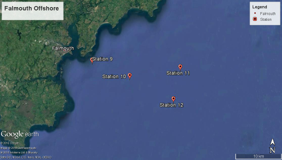
The aim of this offshore fieldwork was to measure and ultimately understand the frontal systems off the coast of Falmouth. Group 9’s offshore fieldwork session took place on 22/06/2016, at 4 stations off the coast of Falmouth, UK. Measurements of physical, chemical and biological parameters were taken at stations 9, 10, 11 and 12
Turner, J. (1980). Small-
At station 9, the graph shows a well-
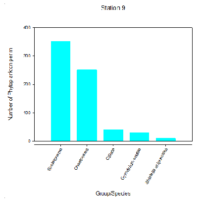
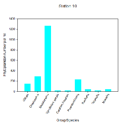
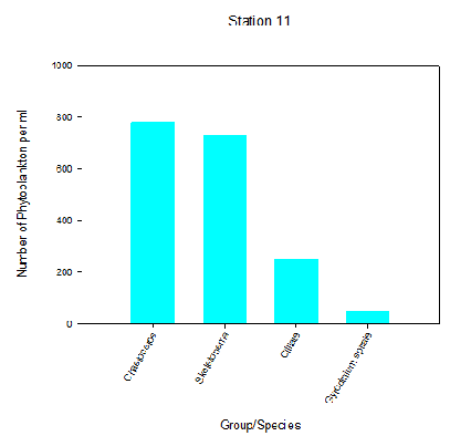
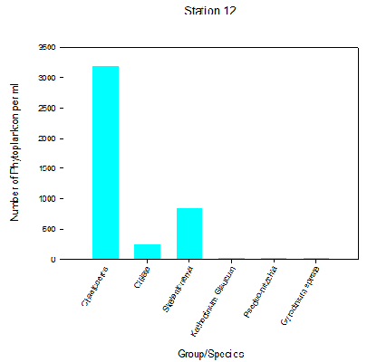
The bar charts represented in the figures below show that there is a diverse range and abundance of groups/species found at different stations that have been sampled offshore. The greatest diversity is found at Station 10 whilst the highest abundance of organisms was located at Station 12 (5610 phytoplankton cells per ml). The diatoms Skeletonema and Chaetoceros were the most dominant species at stations 9, 10, 11 and 12. Truscott (1995) suggests that in temperate North Atlantic coastal waters diatom populations usually experience large peaks in spring and summer often known as blooms. Station 10 and 12 were situated offshore in stratified waters where high levels of chlorophyll were recorded at both stations which conveys recent mixing occurring, resulting in new nutrients available.
In contrast, Station 9 significantly had the lowest abundance of species (950 phytoplankton
cells per ml.) A reason as to why this may have occurred is due to the fact that
Station 9 was positioned furthest away from the front and closest inshore where the
water column was well mixed. The low abundance indicates that the nutrients may have
been utilised throughout the water column due to silicon and phosphate levels being
comparatively low. Moreover, Station 9 predominantly consists of diatoms due to the
water column being well-
All sites demonstrated that the abundance of phytoplankton is highest at lower depths within the stratified water of stations 10, 11 and 12. This is accurate as during the summer months the penetration of light is deeper resulting in phytoplankton being able to photosynthesis further down in the water column (nutricline).
Truscott, J. (1995). Environmental forcing of simple plankton models. Journal of
Plankton Research, 17, pp.2207-
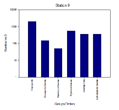
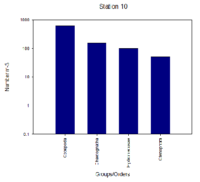
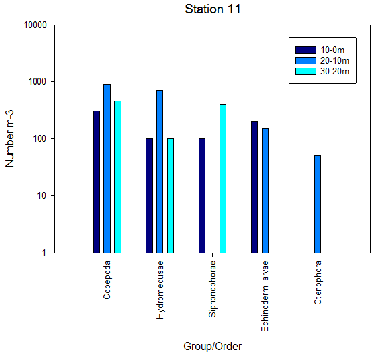
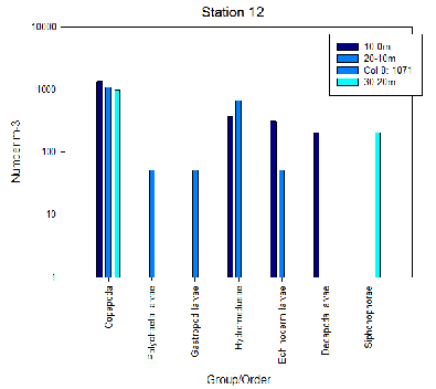
The greatest diversity is found at station 12, the furthest away from shore, which also had the highest abundance of organisms (5458.42 individuals per square metre). In comparison, station 10 had both the lowest diversity and abundance of zooplankton (918.36 individuals per square metre), although this station had the highest diversity of phytoplankton. This result could be due to human error when identifying the zooplankton, as we may have overlooked species. Another possibility would be that at Stations 9 and 10 the zooplankton net was only deployed within the first 10 metres where it was thought the highest amount of chlorophyll was; this meant that species at depth were not recorded.
Across all the stations the most common zooplankton species present were copepoda, hydromedusae and ctenophora. Ctenophora was present in all except station 12. Copepoda were the most dominant species most notable at station 9 and 12, this could be due to their morphology; the shape of their body features aids upward lift and downward sinking during swimming and sinking (Hays, 1994).
Hays, G., Proctor, C., John, A. and Warner, A. (1994). Interspecific differences
in diel vertical migration of marine copepods: The implications of size, colour,
and morphology. Limnology Oceanography., 39(7), pp.1621-
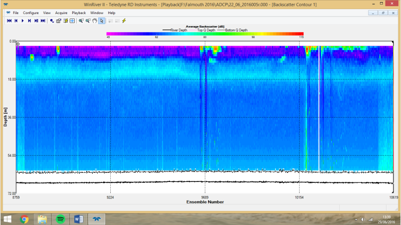
BACKSCATTER:
PROFILE 1
PROFILE 2
PROFILE 3
VELOCITY
PROFILE 1
PROFILE 2
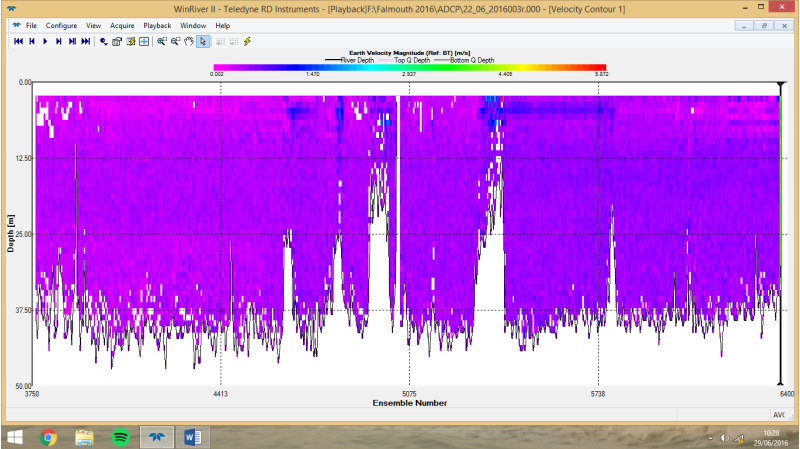
PROFILE 3
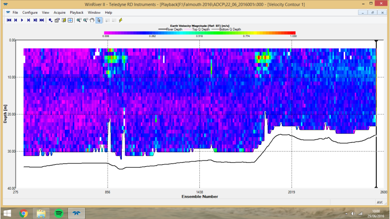
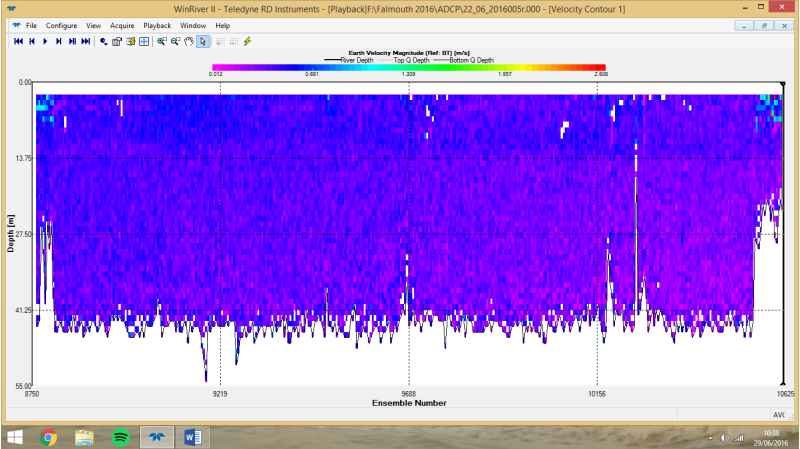
ADCP velocity profiles discussion:
At station 9, there is evidence that there is a stratified water column with low
velocities in the surface layers, faster moving water near the thermocline which
could possibly be due to mixing, before again showing signs of low velocities below
this at approximately 20m. Station 10 seems to be a better mixed water column, showing
the lowest velocity magnitudes of approximately 0.002 to 0.5m/s. There is a small
change between 12 and 25m where the water is slightly faster moving, again around
the thermocline and possible mixing. Station 11 seems to have higher velocity water
than station 10, but deeper in the water column at approximately 41m, the water slows
down, likely due to friction between the seabed and the water. The higher velocity
at the surface at station 11 could be due to the air-
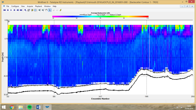
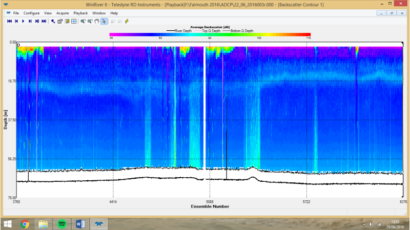
ADCP backscatter profiles discussion:
Figures B1-
The backscatter plots for all 3 stations have a common band of relatively higher
backscatter around 15-
Overcast 8/8 cloud cover, Wind NW F1,Sea state smooth to slight. Tides: High tide: 07:19 (UTC) (4.8m)
Low tide: 13:44 (UTC) (0.8m) High tide: 19:31 (UTC) (4.99m)
| Introduction |
| Methods |
| Results |
| Discussion |
| Introduction |
| Methods |
| Results |
| Physical |
| Chemical |
| Biological |
| Introduction |
| Methodology |
| Results |
| ADCP |
| Richardson |
| Physical |
| Chemical |
| Biological |
| Introduction |
| Methods |
| Poster |