Falmouth 2016 Group 9
Contents:
3. Results
Physical:
A. Salinity Profiles
B. Temperature Profile
C.
Transmission Profiles
E. Flourometery Profiles
F. ADCP Profiles
G.
Richardson Numbers
Chemical:
H. Dissolved Oxygen Profiles
I. Nitrate Profiles
J.
Phosphorus Profiles
K. Silicon Profiles
Biological:
L. Chlorophyll Profiles
M. Phytoplankton Profiles
N.
Zooplankton Profiles
Metadata:
Date: 30/06/16
Time: 07:00-
A70 50°14.392N 005°00.881W
X71 50°13.482N 005°01.002W
B72 50°13.276N 005°01.581W
X73 50°12.454N 005°01.794W
E74
50°11.413N 005°02.749W
G75 50°08.664N 005°01.430W
0716LW, 1321HW (UTC)
Wind: F3 WSW
Cloud: overcast/ broken 6/8 CU,CB.
The Fal estuary is a coastal body of brackish water with a free connection to open sea with not only anthropogenic and fresh water inputs from rivers and streams but also seawater input via the tidal cycles. This gives a habitat over a range of biological, chemical and physical characteristics and our aim was to investigate how these inputs influence multiple factors from the mouth to the upriver fresh water end of the estuary.
Physical, chemical and biological variables were measured at various sites up the Fal estuary, in order to gain a full understanding of the Estuary and its mixing processes. Various sites between the river end member and the sea end member were measured using a CTD, before bottles were taken around depths of interest. These samples and data recorded were then taken back to the lab for analysis and interpretation.
A CTD was attached to a rosette and used to produce a profile of the water column at each station by measuring temperature, density, salinity and chlorophyll. This profile was used to pinpoint areas of interest for deploying Niskin bottles on the return to the boat.
ADCP transects measured the current, flow and area of the area of river using backscatter resonance which could be used to calculate the flushing time and understand mixing patterns. The start and end position of each transect was noted in longitude and latitude.
Niskin bottles we used to collect samples at different depths using several bottles on a rosette and firing at the desired area of the water column. The first sample to be made were for dissolved oxygen to reduce time for change in the collection bottle, these were then processed with 1ml of manganese sulphate and 1ml alkaline solution before being stored underwater. These reagents formed an orange pink precipitate. Another 1 litre sample bottle was then taken with three 50 ml measurements being filtered using syringes into different bottles, plastic polythene, for silicate and dark glass for nitrate and phosphate. The separate plastic bottle for silicate is to prevent contamination or crystallisation from the glass due to being made of similar chemical compositions. The filter papers were then placed in 6ml of acetone for chlorophyll analysis in the dry lab. A sample was also taken for phytoplankton which was dyed with lugols iodide for future analysis. All storing of samples followed scientific protocol to prevent contamination of samples in unwashed bottles.
Zooplankton nets of 200nm mesh and 0.5m diameter were trawled for the same amount of time with a flow meter to calculate the amount of water measured. These were washed into a 100ml sample bottle using a hose and fixed with formalin to prevent changes over night for future analysis
Lab Methods:
Oxygen: Once in the lab, the sealed bottles were taken out of water. The precipitate formed from the previous reagents were broken down by the addition of 1ml sulfuric acid. The bottles were then placed on an automatic titration system using a magnetic stirrer to fully break up the precipitate. The solution was then titrated against sodium thiosulfate which combined with the weight of the glass bottle determined dissolved oxygen concentrations.
Chlorophyll: The 3 acetone sample bottles corresponding to each stations depths were
selected before the removal of filter papers and placed in a 10-
Silicate: 15ml were taken from each sample bottle to be mixed with 6ml of ammonium molybdate and 9ml of a mixed reducing reagent. This consisted of MQ water, metal sulphite, oxalic acid and sulphuric acid solution. One sample out of 5 were repeated to ensure accuracy in spectrophotometry. After a 2 hour period, the samples were placed in the Hitachi U1500 spectrophotometer to measure absorbance. This was calibrated from a set of 6 standards and 3 blanks before being converted to silicate concentrations (µmol/l).
Nitrate: The samples from the field were first filtered again before being injected into a Flow Injection Analysis System to convert nitrate to nitrite. The nitrite concentration was then used to create a nitrate/nitrite ratio that was recorded on a tracer of red and blue peaks. Using standardised peaks these could be compared to attain a concentration (µmol/l) through a calibration curve.
Phosphate: 30ml was measured from each of the field samples before adding 3 ml of mixed reducing agent containing sulphuric acid, ammonium molybdate, ascorbicacid and potassium antimony tartrate solutions. One out of every 5 samples was also replicated to ensure accuracy in spectrophotometry. After a 30 minute period, the samples were placed into a 10cm cell of a Hitachi U1500 spectrometer. A calibration equation was produced from a set of standards and blanks to convert average absorbance to concentration (µmol/l).
Phytoplankton: The samples collected in the field were diluted into 10ml bottles then placed under a microscope and 5 rows of 20 columns were individually counted for species and identified. These were tallied to give an estimate of the dominant species per litre at each station.
Zooplankton: The samples from the field were placed into a cell before being counted for the number and identification of species at each station.
Turner, J. (1980). Small-
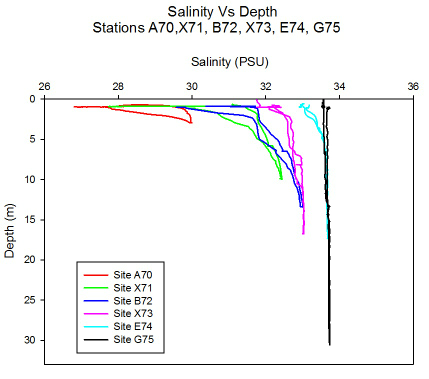
Salinity:
Salinity against depth profiles from the river endmember at Site A70 to
the estuary mouth at site G75 are displayed here. At the fresher end of the stations
although the depth is very shallow a salt wedge estuary is shown due to the low decrease
in salinity at the surface waters with a sharp decrease at depth. This is due to
the less dense lighter fresher input flowing on top of the denser incoming seawater
tide. Compared to station G75 at the estuary mouth where there is almost no change
in salinity throughout the water column due to being well mixed of a high amount
of seawater being diluted by the freshwater input resulting in a high salinity of
33.5 PSU. As the tide becomes a bigger influence further down the estuary, it becomes
less stratified and more mixed resulting in sharper peaks of less change in salinity.
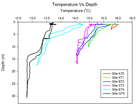
Temperature:
The temperature with depth profiles from the river endmember (Site A70)
across stations to the estuary mouth (Site G75) is displayed. Apart from the obvious
increase in available depth further seaward down the estuary a thermocline becomes
clearer as the 2 bodies of water meet and become stratified. At the fresher end of
the stations at site A70 the temperature decreases more uniformly with a slight thermocline
around 3 meters depth. As we move closer to the estuary mouth a clear thermocline
is apparent such as in Site E74 where there is a gradual temperature decrease to
around 6 meters where there is a sharp decrease indicating passing the thermocline.
This is due to the less dense fresh water flowing on the surface generally being
warmer due to less volume for thermal heating. The denser seawater will be colder
due to a larger specific heat capacity and sinks to the bottom of the water column
hence the sharp decrease.
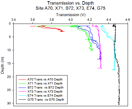
In the graph of transmission vs. depth, we see changes between the stations from the river end member to the sea end member. Towards the river end member at site A70, transmission is low and increases sharply through depth. At site X71 we see a large decrease in transmission values at 1.15m depth, Replicate values at this depth indicate this is likely to be an anomaly in the data. At site B72, transmission increases through depth, however this occurs at a lower rate than at the previous sites. Site X73 is noteworthy as transmission stays almost constant throughout the water column, this is in comparison to site E74 further down the estuary where transmission increases down to approximately 8 metres, after which transmission then becomes relatively constant. Site G75 shows constant transmission to approximately 12 metres depth, this then hits a mild cline where transmission after increases.
Transmission is inversely proportional to turbidity, where turbidity indicates the level of dissolved matter within the water column. In the surface layers towards the river end member, lower levels of turbidity can be attributed to either input of matter from heavy rain or phytoplankton within the water column. In the case of the low transmission observed in station A70, it is likely due to phytoplankton within the water, this corroborates well with the fluorescence and surface phytoplankton bottle samples. High fluorescence in areas of lower turbidity on all other sides supports the hypothesis that phytoplankton is responsible for the high turbidity.
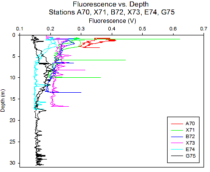
Fluorescence:
Variation in fluorescence trends with depth can be seen between the
6 stations. Station A70, furthest up the estuary, shows peak fluorescence values
at the surface and values decrease with depth. This suggests that the chlorophyll
maximum is at the top of the water column, indicating the highest abundance of phytoplankton
at the surface. The next station down river, X71, features the maximum fluorescence
readings of all the stations, with the maximum being at the surface here also. Contrastingly,
the station closest to the sea (G75) features a maximum fluorescence at around 8m
depth, indicating that the chlorophyll maximum is significantly deeper than at the
stations further up the estuary. The trend appears to be that the chlorophyll maximum
increases in depth as you move towards the ocean. This can be explained by the fact
of increased mixing at the ocean end of the estuary, supplying nutrients from depth.
This increased mixing is also likely to redistribute plankton cells away from the
surface. The phytoplankton will situate at this depth to achieve an efficient balance
of nutrient supply and light availability. Further up the estuary, it’s more likely
that nutrients will be supplied by river water (due to agricultural and weathering
inputs etc.), which lies above seawater due to it being lower density. For this reason,
the nutrients will be greater at the top of the water column. Therefore, phytoplankton
will congregate in the surface layer. The reduced mixing present further up the estuary
will also allow phytoplankton cells to maintain their position in the euphotic zone.
Click to Enlarge.
Click to Enlarge.
Click to Enlarge.
Click to Enlarge.
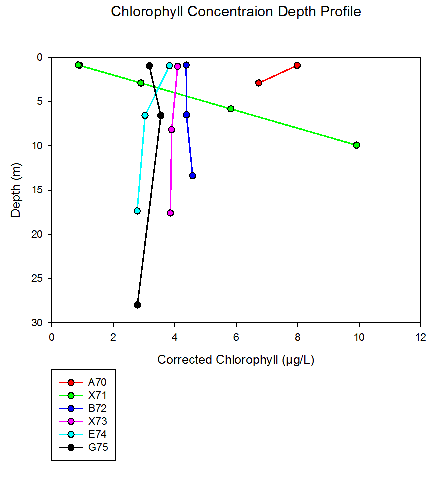
For 4 out of 6 stations, chlorophyll is fairly uniform with depth which would suggest an even distribution of phytoplankton throughout the water column. For the two stations furthest up the estuary (A70 and X71), chlorophyll varies with depth. Station A70 features the highest surface chlorophyll concentration, decreasing with depth but still to a comparatively higher chlorophyll concentration than the rest of the stations. Station X71 shows chlorophyll rapidly increasing with depth. The bottom water chlorophyll concentration here is the highest concentration of anywhere on all of the 6 stations.
The high chlorophyll concentrations at the up-
The effects of mixing are quite significant in the seaward stations, where tidal mixing will be stronger. This mixing will result in a distribution of phytoplankton cells throughout the water column, shown by the uniform chlorophyll concentrations with depth. This is confirmed by the salinity and temperature plots, where stratification is more prevalent up the estuary and plots are more uniform with depth at stations G75 and E74.
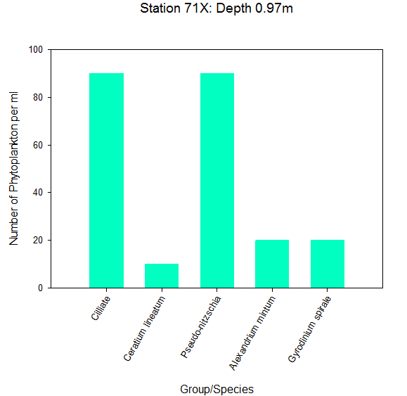
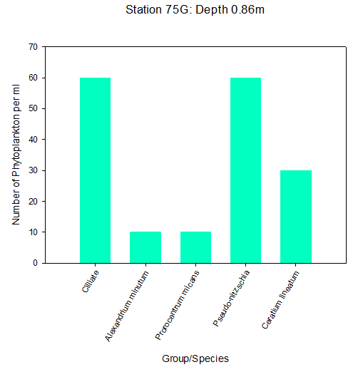
The figures demonstrate that Cilliates and Diatoms were the most dominant groups found at each of the stations with each having a total of 150 phytoplankton cells per ml. Both stations 71X and 75G had a similar range of diversity, although Station 75G had a lower abundance in comparison to Station 71X (170 phytoplankton cells per ml compared to 230 phytoplankton cells per ml). Further up the estuary the abundance of species increase, possibly due to the growth in availability of nutrients. O’Boyle and Silke (2009) suggest that in estuaries the periodic rise and fall of the tide and episodic changes in river flow creates a broad range of conditions that result in greater variation in phytoplankton diversity.
O’Boyle, S. and Silke, J. (2009). A review of phytoplankton ecology in estuarine
and coastal waters around Ireland. Journal of Plankton Research, 32(1), pp.99-
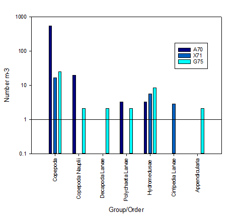
Station A70 recorded the highest abundances of Copepoda with 539.9 individuals per m3. As well as Copepoda Nauplii with 19.40 individuals per m3. This station was the furthest up the estuary and had the highest surface chlorophyll of 8.42m/L in comparison to the other stations which were lower. Some forms of larvae, such as polychaete larvae, were also recorded at this station. Visually the sample taken at Station A70 was significantly more green in colour than the samples from the other stations.
The station with the least abundance and diversity was station X71 which was located
in the mid-
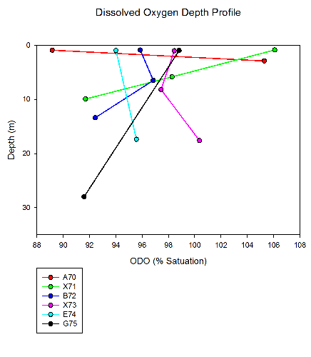
Here the dissolved oxygen as a percentage of saturation is displayed as a profile throughout the water column with depth. The samples were taken from the freshwater endpoint of the Fal estuary at station A70 and at regular intervals down the estuary to the mouth where the endpoint is seawater at station G75. Due to each station having varied maximum depths and number of samples there is too low a resolution to detect a pattern within the dataset. For example, at station A70, only two depths were sampled (surface and bottom). This hinders understanding of what is happening to the dissolved oxygen at the middle of the water column. The middle stations, B72 and X73 show notable bends in the plots. These inflection points may indicate the presence of two separate water masses. These water masses are likely to be river water and seawater, which would feature different dissolved oxygen properties. At the two aforementioned stations, their position in the estuary and time of sampling relative to tide could be characteristic of a stage of stratification, as the flooding tide pushes seawater in, under the less dense river water. Contrastingly, at the stations closer to the open ocean, the plots are much more linear which possibly indicates the influence of more mixing and more dominance from the seawater rather than river water. These stations were sampled at a later (higher) state of tide than the others, and so seawater would have been the main constituent of the water column here.
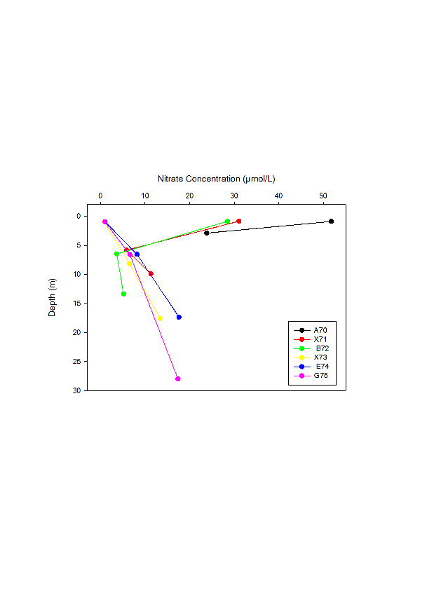
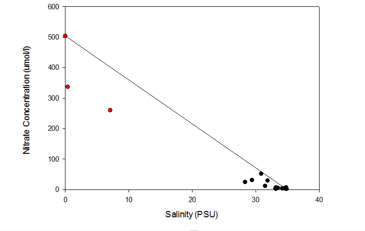
The highest nitrate values have been seen in stations A70, X71,B72 , which are the
stations that were at the source of the Fal Estuary. The highest nitrate values recorded
were found in the surface waters of station A70 where it reached 51.8 (µmol/L). This
is due to the fact that high concentrations of nitrate are found in freshwater and
there was high amounts of freshwater at A70 due to it being low tide when sampling.
Further down the estuary (stations X73,E74 and G75) there is a trend of nitrate concentrations
being low at the surface (approximately 0.8-
Nitrate TDL:
Nitrate TDL: Here the theoretical dilution line for nitrate is displayed between
the river and estuary mouth endpoints of the Fal estuary. From the TDL we can see
most of the points lie below the line indicating non-
Nitrate sources consist of natural forms such as waste from natural animals but also
anthropogenic inputs such agricultural and livestock run off but this has not seemed
to have a large impact on the Fal estuary at this time of year due to the lack of
evidence of non-
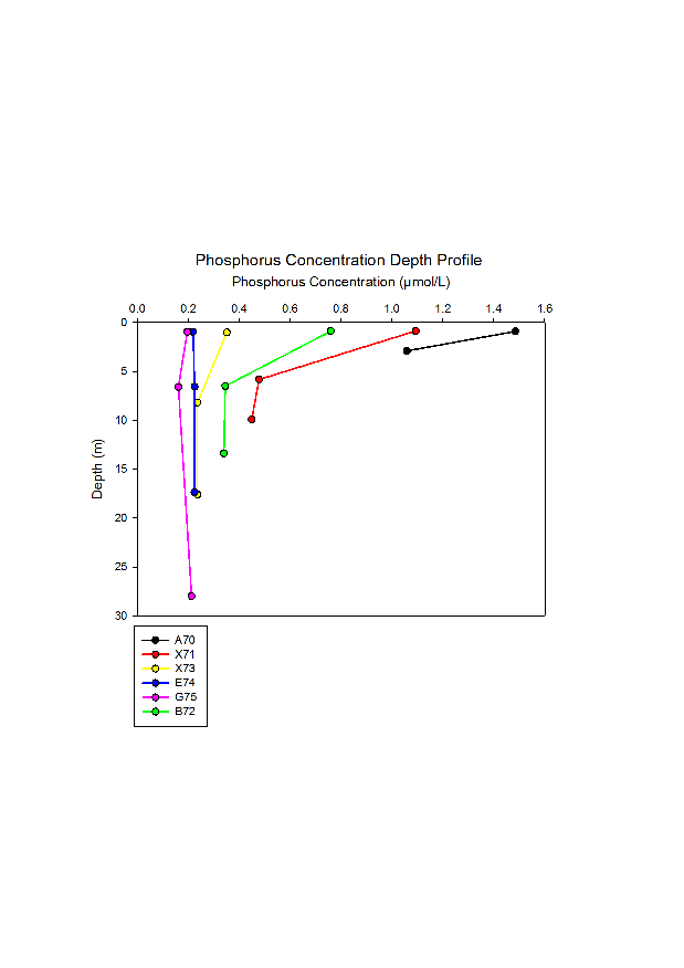
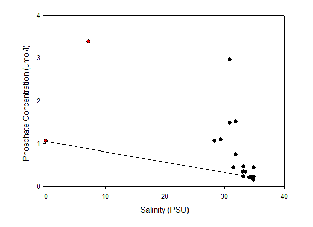
Here the Phosphate Concentrations of the Fal estuary from stations at the freshwater endpoint to the seawater endpoint at the estuary mouth. As shown by the graph as we move away from the river end, phosphate surface concentration decreases from 1.5 µmol/L at station A70 to 0.2 µmol/L at station G75 at the estuary mouth. Where the seawater and fresh water are well mixed at the mouth of the estuary, phosphate remains fairly constant throughout the water column. This is evident in stations E74 and G75 with the straight lines. Towards the river endmember there appears to be more stratified with a slow decrease in concentration such as 1.5 µmol/L to 1.05 µmol/L at station A70 indicating 2 bodies of water. This could be investigated further with a higher resolution of samples with depth to highlight a nutricline in the water column.
Phosphate TDL:
The TDL profile for Phosphate shows a very non-
The graph illustrates that further up the Fal estuary towards Station 70A the concentration
of Silicate increases due to a higher percentage of river flux delivering fresh nutrients
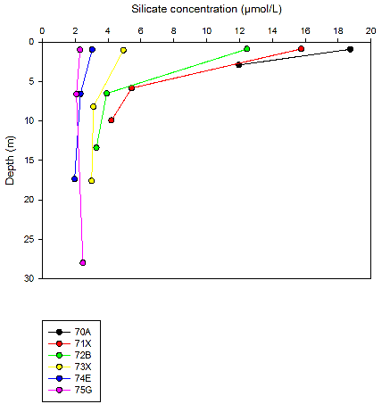
to the estuary. The maximum silicate concentration was found at station 70A with
a concentration of 18.7 µmol/L. The results also indicate that the lowest concentration
of silicate is found at Black Rock (Station 75G) with 2.3 µmol/L as this is situated
further down the estuary. At station 74E and 75G the dissolved silicon decreases
slightly at the surface and then remains fairly consistent throughout the water column
between the depths ranging from 7m-
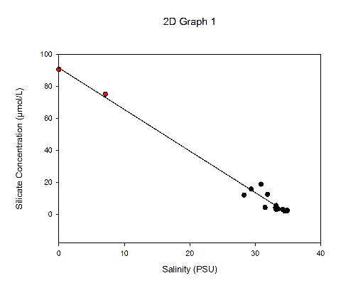
Silicate TDL-
Dickie, B. (2010). Lecture 14: Behaviour of Chemical Species During Mixing. Retrieved
from Southampton School of Ocean and Earth Sciences: http://www.soes.soton.ac.uk/teaching/courses/oa217/chemicalprocesses-
Voss, M., Baker, A., Bange, W., Conley, D., Cornell, S., Deutsch, B., Engel, A.,
Ganeshram, R., Garnier, J., Heiskanen, A., Jickells, T., Lancelot, C., Mcquatters-
Smith,J.D, Longmore,R.L ‘Behaviour of phosphate in estuarine water’ Nature 287,5322-
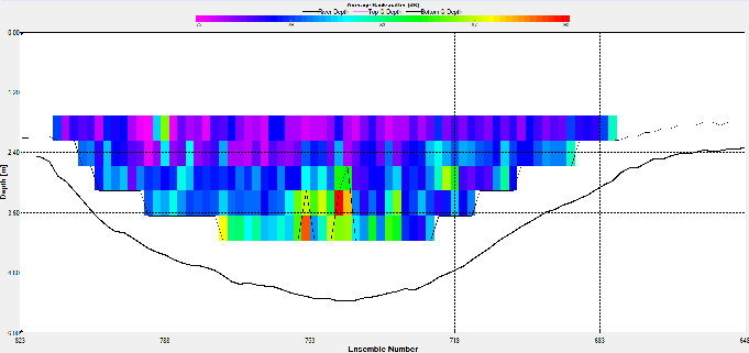
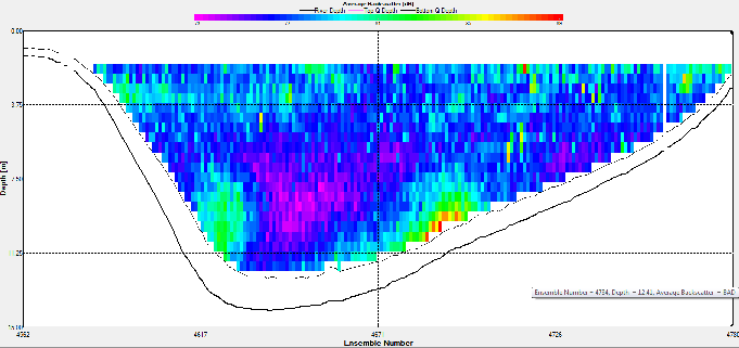
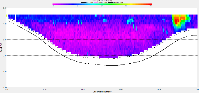
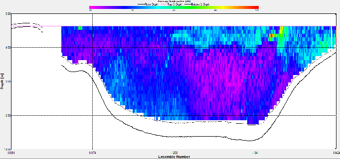
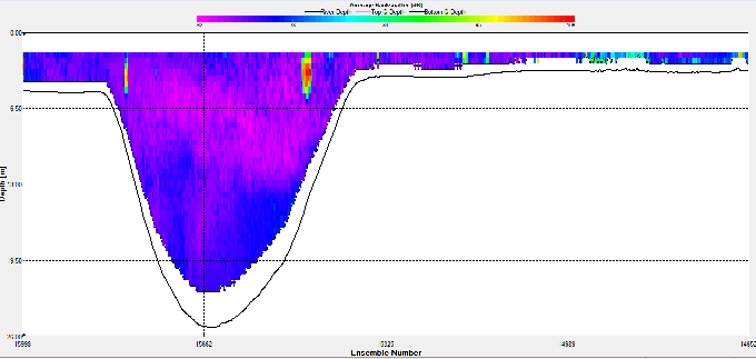
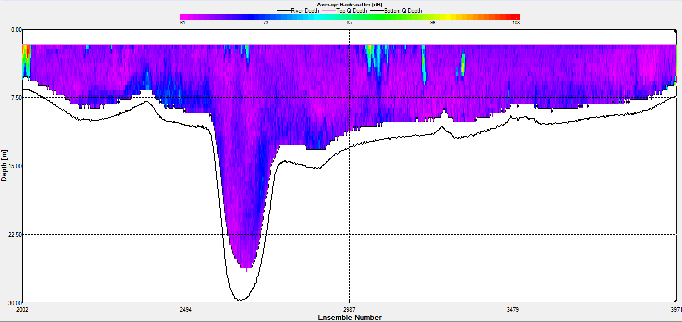
Backscatter results/discussion:
At station A70, the ADCP backscatter data shows highest backscatter at depth, and lowest backscatter at the surface. This trend is not as clear for station X71, where regions of high backscatter are observed at the surface as well as depth, with a low backscatter region in the centre of the water column. Station C72 shows comparatively low backscatter throughout the water column, apart from a region of high backscatter at the surface, near the river bank. E73 shows evidence of low backscatter throughout the water column apart from a region of comparatively higher backscatter on the eastern edge of the estuary in the surface layer. E75 has fairly low backscatter throughout the water column. G75 also has relatively low back scatter throughout the water column, apart from a surface areas with higher values.
Backscatter in the ADCP data is likely to be representative of two things; the presence of zooplankton and other marine organisms and the presence of suspended matter in the water column. The influence of suspended matter on the backscatter readings will be more apparent at the bottom of the water column. This explains the high backscatter values seen in some of the shallower stations further up river, where bottom friction would be stronger, increasing turbidity. This affect is less apparent at the deeper stations closer to the sea, where the flow is slower and less focussed. The backscatter regions in the surface layers at these stations are possibly due to the presence of zooplankton in the water column. In the middle stations, the effects of both of these backscatter sources are apparent. `
A70
X71
C72
X73
E74
G75
Click to Enlarge.
Click to Enlarge.
Click to Enlarge.
Click to Enlarge.
Click to Enlarge.
Click to Enlarge.
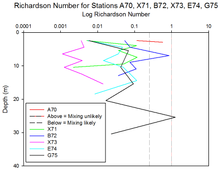
The Richardson numbers produced for stations on the estuarine fieldwork feature a
variety of mixing-
Click to Enlarge.
| Introduction |
| Methods |
| Results |
| Discussion |
| Introduction |
| Methods |
| Results |
| Physical |
| Chemical |
| Biological |
| Introduction |
| Methodology |
| Results |
| ADCP |
| Richardson |
| Physical |
| Chemical |
| Biological |
| Introduction |
| Methods |
| Poster |