
The views expressed on this website are not those of the University of Southampton or the National Oceanography Centre Southampton
Offshore
A
B
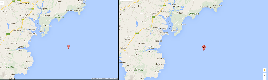
Figure 3.(5) A Shows the location of the initial CTD deployment from off-shore deployment. B Shows the 4 CTD deployments for the off-shore time series conducted, the locations were kept as close together as possible but it was not possible to stay in exactly the same location. For each deployment. Specific locations of each deployment are given in table 2.
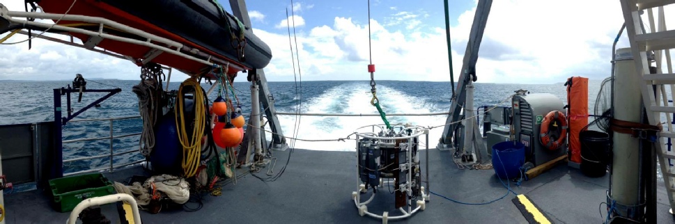
An off shore-time series was conducted from the vessel Callista in the location(s) shown in figure 3. The time series consisted of four CTD deployments every hour with five depths of interest sampled using niskin bottles for each deployment. Water samples were taken from the niskin bottles for later analysis of silicon, nitrate, phosphate, chlorophyll, zooplankton and phytoplankton; a plankton net was towed vertically to collect samples for each station. Stationary transects were also taken each time the CTD and plankton net entered the water.
Methods
The CTD rosette was deployed four times, every hour at the locations given in Table 2, the temperature, salinity, fluorescence, PAR/irradiance, cDOM, turbidity, beam transmission and density were all recorded. Five depths of interest were chosen to sample, Niskin bottles were then fired at these chosen depths as the CTD was brought back up through the water column to the surface. Water samples were processed and stored in the same way and nutrient, oxygen, chlorophyll concentrations were analysed using the same standard methods as those described for the Fal Estuary water samples. The zooplankton and phytoplankton were also stored and analysed in the same way described for the Fal Estuary samples. Sigma Plot was used to process the CTD data and a decision was made to only plot the up cast data of the CTD as this was when the Niskin bottles were fired. Additionally, to collect data and samples from the surface of the water column a depth of 4m was targeted in order to avoid wave action.
A
B
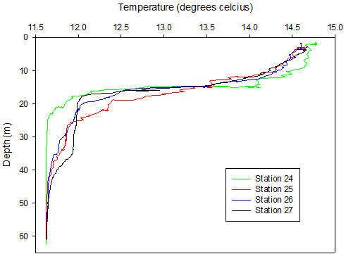
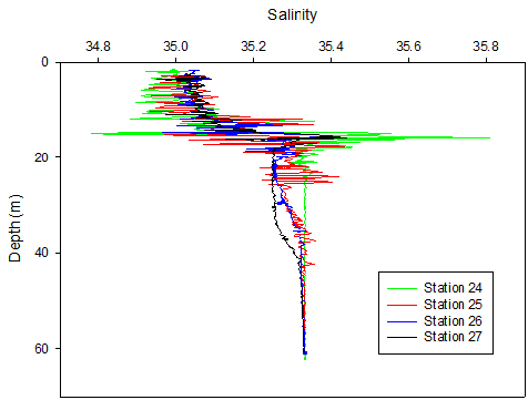
Figure 28. A Temperature depth profile and B salinity depth profile obtained from the upward cast of the CTD for each station during the offshore survey on 25/06/2016, locations of stations are given in table 2.
Figure 37. Fluorescence depth profile taken from the upward cast of the CTD from each station during the offshore survey on 25/06/2016.
Table 2. Metadata for offshore sampling on 25/06/2016, location is given for each station along with depth, weather and duration of CTD deployment.
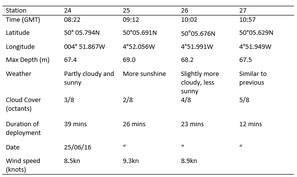
The time series showed temperature to decrease with as well as exhibiting variation in stratification, despite end members (at surface and depth) remaining relatively constant at around 14.7°C and 11.6°C. The initial measurement (Station 24 08.22 GMT) revealed a strong thermocline starting at 14m and ending abruptly at 16m. At Station 25 (09.12 GMT) the water column appeared to be more mixed, as the rate of change of temperature decreased, now spanning 20m as opposed to 2m as seen at Station 24. At Station 26 (10.02 GMT) the thermocline was slightly less mixed. The final measurement (Station 27 10.57 GMT) showed the water column to be stratified again with a sharp region of change extending only 4m, similar to Station 24.
The movement and mixing of the thermocline is evidenced in Fig 28a. Figure 28b shows salinity spikes as a result of the lag in response time between the thermistor and conductivity sensor on the CTD. Conductivity is affected by temperature therefore the spikes of larger magnitude are proportional to the thermal gradients, hence why the largest spikes are seen at the thermocline (15m). Across all stations the surface salinity is ~35 and increases to 35.3 at the seabed (61m), as expected for an offshore location as fresh riverine water is diluted. A halocline is also evidenced on Fig 28b at 14m, which is a similar depth to the thermocline. As with temperature the most stratified station is 24 which reaches a salinity of 35.3 at ~22m, all other stations reached this salinity at ~45m after some light mixing between 25-40m.
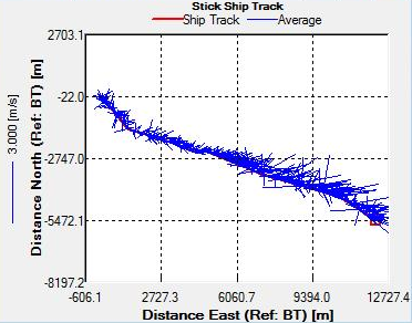
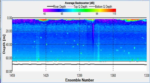
Figure 31. ABackscatter contour plot for stationary transect at Station 24 at 09:00, obtained by ADCP
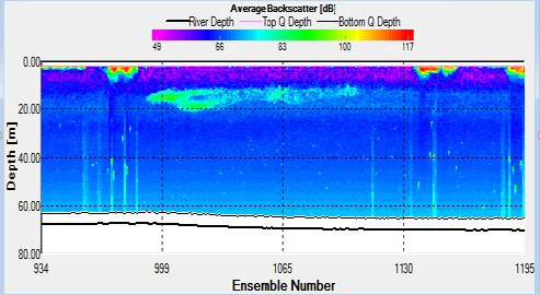
Figure 30. Backscatter contour plot for stationary transect at Station 24 at 08:44GMT, obtained by ADCP
Strength of flow reduced considerably at Station 24, for both the transects taken during the CTD sample and the plankton net trawl, between 08:44 and 09:00. Both transects also exhibited high surface backscatter. The backscatter plot during the CTD transect also showed an isolated area of high backscatter between 10 and 20m.
A patch of strong backscatter is also visible between 10 and 20m at 09:26, corresponding to a reversal in direction of total water flux. High surface backscatter values returned after 10:13. Velocities of around 0.5m3/s could be seen progressing in direction from around 90O anticlockwise to true North to 180O anticlockwise to true North.
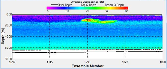
Figure 32. Backscatter contour plot at stationary transect at Station 25, obtained by ADCP.
Figure 29. Ship track data for spatial transect between the marina and Station 24, obtained by ADCP
The concurrence of both the halocline and thermocline suggests the presence of two water bodies; a warmer, less saline body in the upper 20m and a cooler, more saline body between 20-60m. The short term (hourly) variation in stratification may be linked to the tidal stream of Falmouth Bay. Although generally water is well mixed near the coast and becomes stratified offshore, Falmouth experiences patchiness in stratification due to varying depths, tidal influences and the advection of structures from the estuary. The tide moves along the South coast in a North East East direction and leaves in a Southwest direction when the tide ebbs. On the 25/06/2016 it was spring tide and high tide occurred during the middle of sampling at 09.14 (39). The strong stratification seen in both the first and last measurements, and the turning of the tide during the middle of the sampling (evidenced in the ADCP WinRiver stick ship track) could imply that the same stratified structure was measured as it passed and returned through our position, once with the flooding tide and once with the ebbing tide. The same could be said for the well mixed structures measured at Station 25 and 26. This theory may also be evidenced in the ADCP backscatter data that depicts the progression of a parcel of water with higher scattering properties (inshore with the flood tide and offshore with the ebb tide) (Fig ? – ask lara/sam for specific one if not sure). Alternatively the changes in stratification seen could be due to internal waves. Navrotsky (2013) states that in shallow waters high frequency internal waves can appear and disappear in packets depending on the phase of the barotropic tide (40). Such internal waves would disturb the thermocline and bring about mixing, especially if they break and cause turbulence.
A
B
C
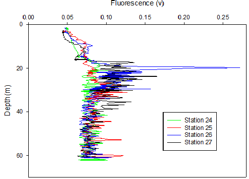
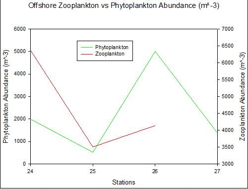
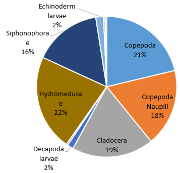
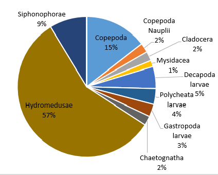
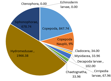
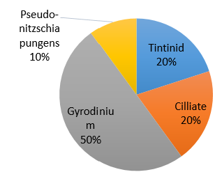
Figure 39. Zooplankton species composition at one site (Bi) offshore over a time series (Station 24 [A], station 25 [B], station 26 [C]). Pie-charts display identified zooplankton species to the highest taxa possible using identification catalogues. Percentages represent the calculated species composition per ml of each individual station. Samples collected using a trawl net between 15-30m.
Figure 38. Total phytoplankton and zooplankton abundance 4 stations in a time series at the offshore site Bi. Abundance calculated using a 1000ml sample collected from each site using a discrete sampling trawl net between depths 15-30m.
A
B
C
D
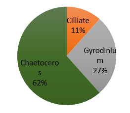
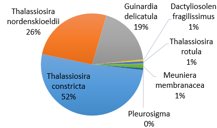
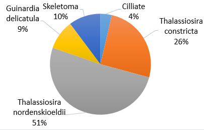
Figure 40. Phytoplankton species composition at the offshore site Bi over a time series (Station 24 [A], station 25 [B], station 26 [C], station 27 [D]). Pie-charts display identified phytoplankton species to the highest taxa possible using identification catalogues. Percentages represent the calculated species composition per ml of each individual station. Samples collected using a discrete sampling trawl net between 15-30m.
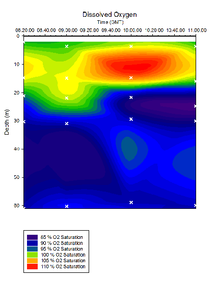
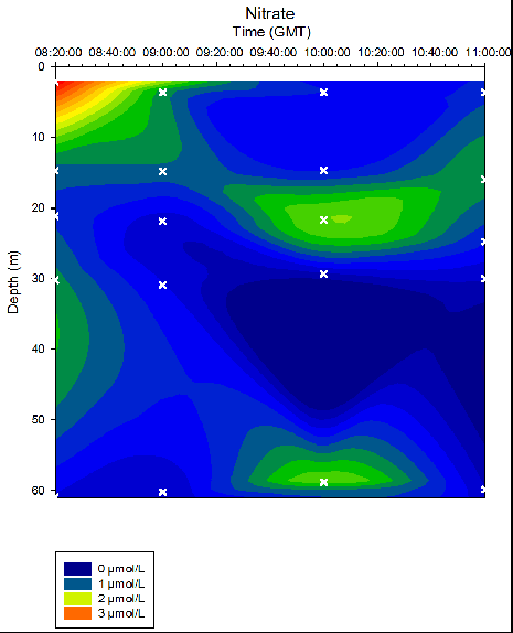
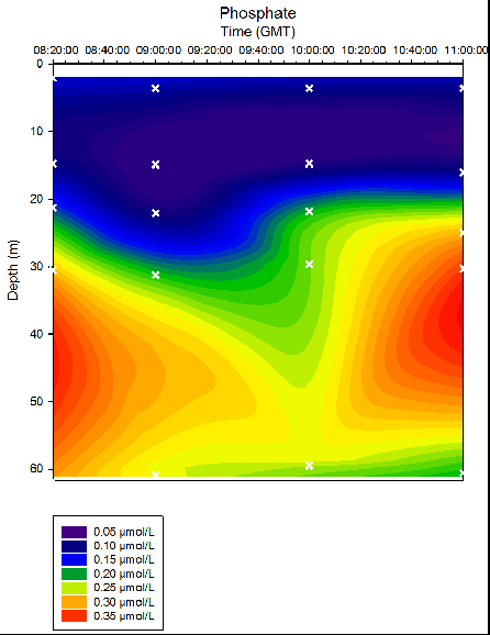
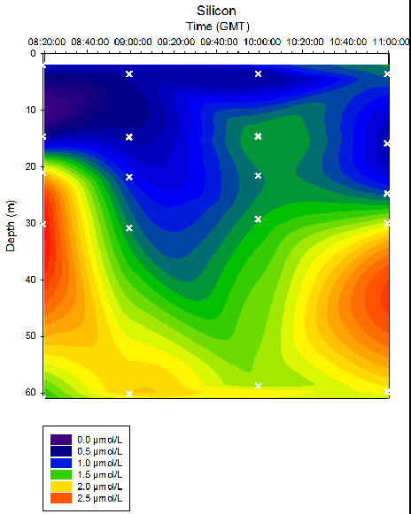
Figure 33. Dissolved Oxygen in time series at location B offshore of Falmouth (50° 05.794N 004° 51.867W). Measurements collected in Niskin bottles from 08:20 to 11:00 (GMT) on 25/06/16. Time and depth of each measurement indicated by white crosses. Dissolved O2 determined in the laboratory on the 27/06/2016.
Figure 34. Nitrate concentrations in time series at location B offshore of Falmouth (50° 05.794N 004° 51.867W). Measurements collected in Niskin bottles from 08:20 to 11:00 (GMT) on 25/06/16. Time and depth of each measurement indicated by white crosses. Nitrate determined in the laboratory by flow injection on the 27/06/2016.
Figure 36. Dissolved silicon concentrations in time series at location B offshore of Falmouth (50° 05.794N 004° 51.867W). Measurements collected in Niskin bottles from 08:20 to 11:00 (GMT) on 25/06/16. Time and depth of each measurement indicated by white crosses. Dissolved silicon determined in the laboratory by colourimetry methods on the 27/06/16. Repeats taken every 5 measurements.
Figure 35. Phosphate concentrations in time series at location B offshore of Falmouth (50° 05.794N 004° 51.867W). Measurements collected in Niskin bottles from 08:20 to 11:00 (GMT) on 25/06/16. Time and depth of each measurement indicated by white crosses. Phosphate determined in the laboratory by colourimetry method on the 27/06/16. Repeats taken every 5 measurements.
As depth increased, silicon concentrations generally increased. Stations 24 and 27 exhibit the most variation in silicon concentrations over depth, with maximum silicon depths of 25-40m and 40-50m respectively. Over time, the maximum nitrate depth decreased from ~ 3m at 08:20 to ~21m at 10:00, with a further nitrate maximum at ~60m. Due to the limited number of samples at each station, it is not possible to conclude whether this data is a true representation of the water column. As depth increased, phosphate concentrations generally increased. Stations 24 and 27 (taken at 09:00GMT and 10:00GMT) exhibit strong phosphate maximums at the depths 40-50m and 35-45m respectively. At Station 25 (taken at 09:00) the surface layer where phosphate is low is approximately 10m deeper than the majority of stations profiled.
Fig 37 shows a period of relatively constant fluorescence from the surface to ~20m. At this depth a region of sharp increase was noted after which the fluorescence settled to remain fairly constant once more. The greatest fluorescent peak occurred at ~20m at 10:00. As depth increased, dissolved oxygen saturation decreased. Dissolved oxygen is shown to have a maximum at ~10-15m at each time station, the greatest of which occured at 10:00.
Discussion
The peak in fluorescence and decrease in transmission at approximately 20m (Figure 37) indicates the presence of a chlorophyll maximum just below the thermocline. This is likely to be a result of the presence of phytoplankton due to the favourable conditions of a balance between limiting factors; light and nutrient availability. At the surface there is ample PAR but nutrients are limiting and vice versa at depth hence why the base of the thermocline provides ideal conditions. Additionally, the stratification leads to high concentrations of upwelling nutrients forming at the base of the thermocline and therefore an increase in biological activity occurs.
Throughout all time stations, silicon and phosphate concentrations are lowest at the surface and greatest at depth (Fig. 35, 36). This may be due to the uptake of these nutrients by phytoplankton. Silicon is taken in by siliceous diatoms which use silicon to produce their testes. Phosphate is used by organisms to produce DNA, proteins and sugars. In particular, phosphate is a key component of ATP, which is universally used as an energy source for metabolic reactions. This is supported by the data depicted in Figure 33, which shows highest dissolved oxygen concentrations in the surface waters compared to at depth. Though this may reflect the interactions between the atmosphere and seawater, it is more likely that this is reflecting high photosynthetic rates at the surface, due to increased abundance and activity of phytoplankton.
At Stations 24 and 27, there is strong stratification of silicon concentrations with depth, and maximum silicon depths are clearly discernible at depths of 30-40m and 40-50m respectively (Fig. 36). However, this stratification is less obvious at Stations 25 and 26, at which the distribution of silicon within the water column is seen to be more uniform. A similar pattern is seen with the phosphate profiles (Fig. 35); at Stations 24 and 27 clear maximum phosphate depths were observed at 40-50m and 20-30m respectively, whereas at Stations 25 and 26, no apparent maximum depths can be observed. This supports the hypothesis suggested in the physics discussion that a period of mixing within the water column occurred during Station 25 and 26, as a consequence of the turning of the tide.
Hydromedusae was found to be the most dominant zooplankton throughout all the stations and can sometimes reach considerable numbers [25]. Predation by Hydromedusae can substantially affect the abundance of zooplankton [26] as well as fish eggs and larvae [27] which may suggest why other species of zooplankton have lower abundances at each station and why there are such low percentage abundances of Decapoda, Polychaeta and Gastropoda larvae at station 25 where Hydromedusae is most dominant (Fig. 39). Some species of Hydromedusae have been found to feed almost entirely on copepods [28]. This corresponds to the negative correlation between Hydromedusae and Copepoda percentage abundance across stations 24 and 25 (Fig. 39). Despite this, the percentage abundances for smaller organisms such as Copepoda nauplii may be inaccurate. 40% of copepods sampled between 1992 and 2001 were nauplii. It is therefore important to choose a mesh size that doesn’t exclude youths [30]. However, the mesh size used in our method was 200 microns which is likely to catch only 7% of numbers between 200micron and 20mm body length [30].
Gyrodinium is a dinoflagellate, forming common blooms in European waters [31]. The toxic blooms are triggered by anthropogenic and natural inputs of iron. The high percentage of Gyrodinium at stations 24 and 25 (Fig. 40) could be a result of the waste discharge from the old mining industry into the Fal estuary [32]. The species ability to position itself in the water column for favorable light conditions reflects the high abundance collected in samples [33]. Preference for euryhaline and eurythermal waters suggests the species can outcompete other phytoplanktonic species when environmental conditions change. Equally, the ability for Gyrodinium species has the capacity to store phosphorus and be motile in the water column makes them well adapted to more oceanic waters [34].
The lack of Gyrodinium at stations 26 and 27 can be due to identification error as more than one person was counting plankton individuals from the samples. Equally, the trawl net will not have sampled the exact location as the previous samples, and the Gyrodinium population may have been missed.
As the largest of the marine planktonic diatom [35] Chaetoceros could be expected to outcompete other producers in the presence of sufficient nutrients. One factor that may contribute to a lack of dominance in stations other than 25 (Offshore Location Bi at time 10:13) could be the presence of well-defined thermocline structures, that restrict the movement of the diatoms vertically through the water column. Furthermore, research suggests that the Chaetoceros is relatively unaffected by temperature and salinity ranges in mid-latitude [36] waters such as those surrounding Falmouth bay, further suggesting it might be expected to be present in each of the time varying stations. Altogether, the exclusive presence of Chaetoceros at Station 25 is expected to be a result of human error in identification.
The ability of ciliates to ingest nano-sized food particles [37] provides another source of energy to them other than production, enabling them more growth stability in the absence of nutrients ahead of other autotrophs. Also, smaller ciliates have higher growth rates than algae of the same cell volume [38], further enabling them to out compete other phytoplankton. Once again the unexpected disappearance of a Ciliate population at station 26 suggests considerable error in the species identification and net trawling methods.
The intense dominance of certain phytoplankton due to physical advantages, has allowed these species to easily out compete weaker ones, sometimes to the level of complete expulsion. This can be seen in the small diversity values exhibited in the plankton identification.