
The views expressed on this website are not those of the University of Southampton or the National Oceanography Centre Southampton
Fal Estuary
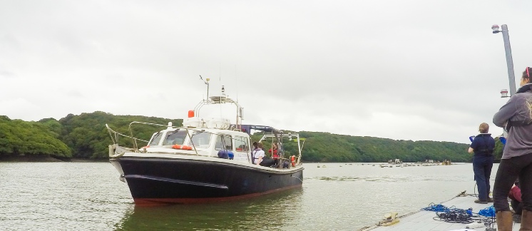
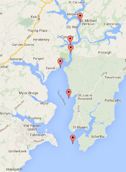
Six sites on the Fal estuary were sampled using the vessel Bill Conway, to look at: temperature, salinity, chlorophyll, silicon, nitrogen, phosphate, dissolved oxygen and plankton distributions For each station a secchi disk was also deployed. The sites which were sampled are shown in figure 2 and were sampled consecutively starting at A1 and working down to G6 to account for the tide times; low tide occurred at 11:29 GMT and the tidal period was peaking in the spring phase. A relatively large tidal range of 4m was observed.
Methods
Water samples from various depths of the water column were collected using Niskin bottles attached to a CTD rosette. Depths sampled were classified as ‘deep’, ‘middle’ and surface with specific depths recorded. Two bottles were fired at each depth and water was first transferred into sealed glass bottles and stored underwater to later determine oxygen concentration. Water was then transferred to other glass bottles for nitrate and phosphate analysis and plastic bottles to later determine silicon. Three replicate 50 ml samples from each depth were filtered using filter paper and syringe, the filters were stored in 6ml of acetone and kept in a freezer for 24 hours for later analysis of chlorophyll concentration.
A plankton net with 200µm mesh was towed horizontally through the surface at station A1, C3 and G6 and water samples collected in bottles and fixed with 10% formalin for zooplankton analysis. At each station 100ml of sample water was transferred to glass bottles containing Lugols iodine to fix any phytoplankton for later analysis.
Figure 2.(5) Shows the six sites which were sampled on the Fal Estuary. A1 - (50°14.394 N, 5°00.888 W.) B2 - (50°13.328 N, 5°01.568W). C3 - (50°12.927 N, 5°01.568 W). D4 - (50°12.927 N, 5°02.330 W). F5 - (50°10.834 N, 5°01.716 W). G6 - (50°08.718 N, 5°01.430 W).
Chemical Analysis
The nitrate concentration of samples was determined in the laboratory using the Johnson and Petty (1983) Flow injection analysis method. (6) Dissolved oxygen was determined using the standard Graffhoff, Kremling and Ehrhardt 1999 method (7) .The chlorophyll, phosphate and silicon concentration were determined using the standard methods outlined by Parsons, Maita and Lalli (1984)(8). The bench top UV fluorometer (10 AU, Turner designs) was used in chlorophyll analysis.
Biological Analysis
The seawater-lugols iodine mixture was reduced down to 10ml to concentrate the phytoplankton, this was then transferred to a 1µm Sedgewick-rafter counting chamber, species were counted and identified to determine the cell concentration per ml. 10ml of water collected from the zooplankton net was analysed to determined the species and abundance of plankton. The plankton per m3 was then calculated from this.
Table 1. Metadata for the Fal estuary on 20/06/2016 during sampling. Stations are given along with information on weather, depth of location and time of sampling.
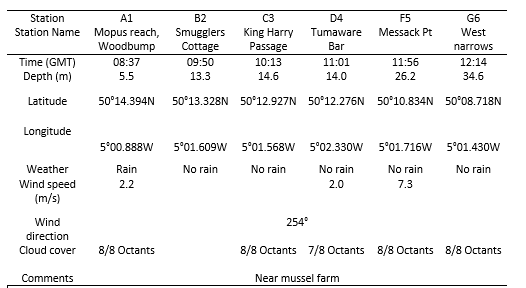
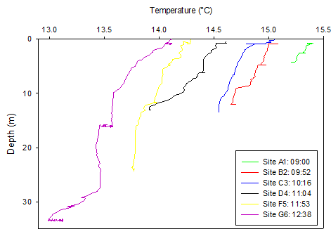
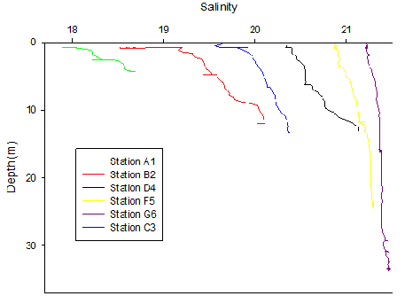
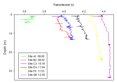
Figure 3. Temperature (°C) depth profile for all sites along the Fal Estuary on 20/06/16. Times indicate the time CTD was deployed at each site. Only the upcast data is plotted.
Figure 4. Salinity depth profile for all sites along the Fal Estuary on 20/06/16. Only the upcast data is plotted.
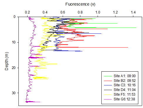
Figure 5. Transmission (volts) depth profile for all sites along the Fal Estuary on 20/06/16. Transmission not yet calibrated for by the chlorophyll values. Only the upcast data is plotted.
Moving down the estuary the maximum depth increased whilst the temperature generally decreased throughout the water column. There was an overall 1.292 °C decrease from site A1 (15.393°C) to site G6 (14.101°C) at the surface. At sites A1-C3, in the upper part of the estuary, there was less temporal variation with depth compared to sites D4-G6. For example, at site A1 there was a difference of 0.165°C between the surface and deep waters whereas for site G6, there was a difference of 0.991°C. Sites A1 and B2 showed an obvious thermocline compared to the other sites where there was a gradual decrease in temperature with depth.
Salinity increased both vertically with depth and laterally with movement downstream. There was an overall difference of 2.83 between the surface water salinity from sites A1 (18.63) to G6 (21.46). However, with movement along the estuary, variation in salinity from the surface to the deeper water decreased. For instance, at site A1 there was a difference of 0.63 between the surface and 4.25m, whereas at site G6 there was a difference of 0.24 between the surface and 33.62m.
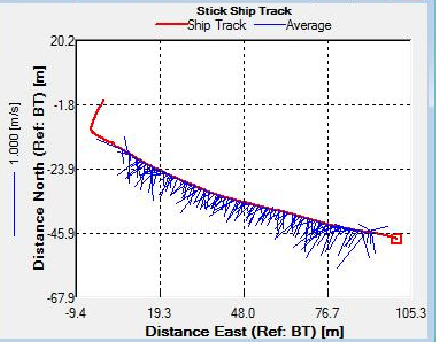
Figure 6. Stick Ship Track at Station A1, indicating the direction and velocity of the transect across the estuary
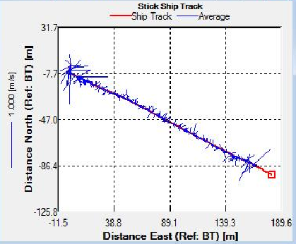
Figure 7. Stick Ship Track at Station D4, indicating the direction and velocity of the flow
A
B
C
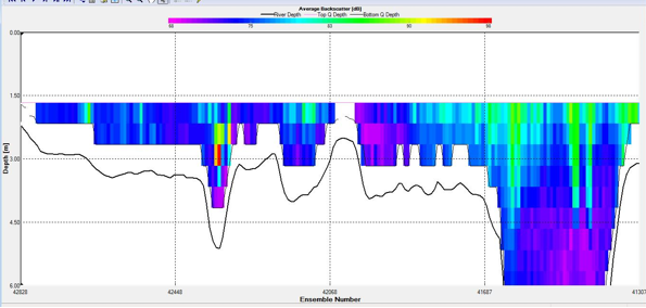
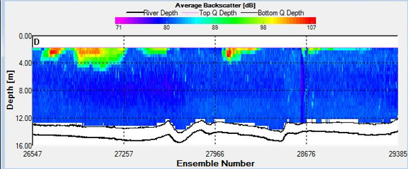
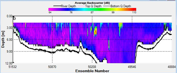
Figure 8. Backscatter Contour Plots taken at spatial transect across the estuary at A) Station C3, B) Station F5, and C) Station G6
Sites C3 and D4 were sampled as the tide reached it’s lowest point and as it began to turn respectively. This is evidenced on the Stick Ship Track figures. Station C3 in particular exhibited patches of high backscatter at the surface, whilst D4 exhibited less obvious scatter.
Spatial transects indicated upstream water flux at site F5, accompanied by a large volume flux value across the mouth of the estuary of 932.7 m3/s as the tide began to flood. Volume flux further increased to 4261.8m3/s upstream at Blackrock site G6. High backscatter values were relatively consistent across the upper 3m at F5, while patches of extremely high backscatter were found both at the surface and in the upper column at G6.
A1
D4
C3
B2
F5
G6
Figure 9. Nitrate concentration for three different depths at each site surveyed on the Fal Estuary.
Figure 10. Phosphate concentration for three different depths at each site surveyed on the Fal Estuary.
Figure 11. Silicon concentration for three different depths at each site surveyed on the Fal Estuary.
Silicon concentrations were seen to decrease as depth increased for all sites (Fig. 11). As the location of the sampling sites moved downstream, silicon concentrations decreased. The highest silicon concentrations were seen at site A1 (8.18mmol/L maximum). Site G6 showed the least change in silicon concentrations with depth.
Nitrate concentrations were seen to decrease as depth increased for all sites except site F5 (Fig. 9). As the location of the sampling sites moved downstream, nitrate levels decreased. The highest nitrate concentrations were seen at site A1 (16.97mmol/L maximum). Site F5 showed the least range of nitrate concentrations with depth.
Phosphate concentrations were seen to have little variation with depth for all sites except sites A1 and B2 (Fig. 10). As the location of the sampling sites moved downstream, phosphate levels decreased. The highest phosphate concentrations were seen at site A1 (1.07mmol/L maximum). Site G6 showed the least range in phosphate concentrations with depth. Mixing diagrams have not been included because the range of salinity was too limited for a meaningful interpretation when compared to the theoretical dilution line. Therefore it is not possible to tell if any of the nutrients present exhibit non-conservative or conservative behaviour.
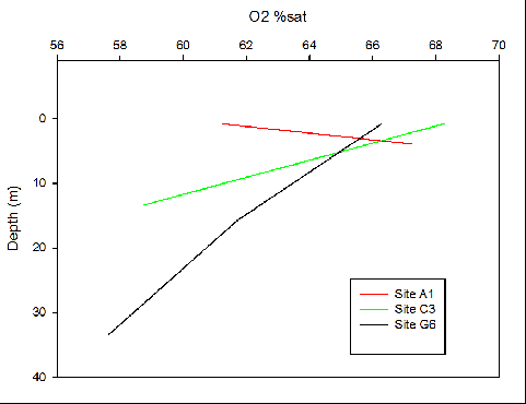
Figure 12. Oxygen saturation with depth profile at 3 sites along Fal Estuary where A1 is upper estuary, C3 is mid estuary and G6 is lower estuary.
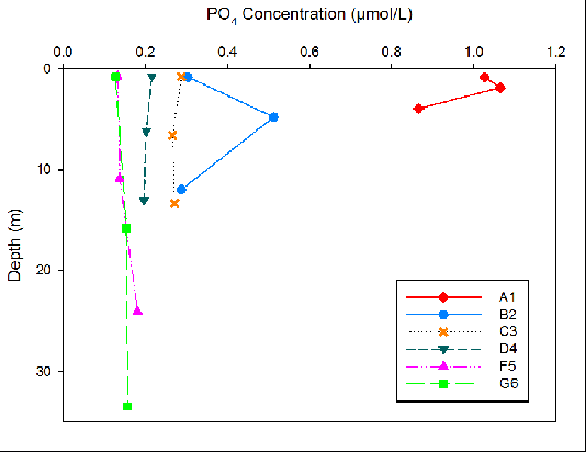
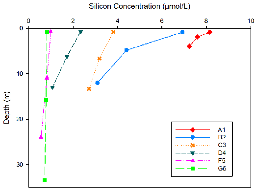
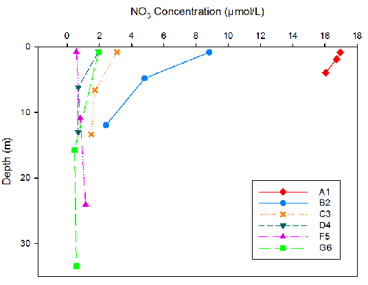
Figure 14. Depth profile for all sites along the Fal Estuary on 20/06/16. Times indicate the CTD deployment at each site. Only the upcast data is plotted.
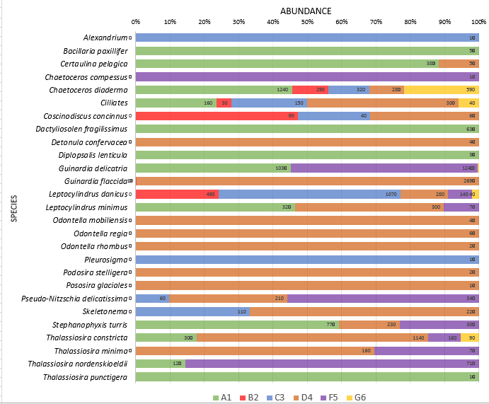
Figure 13. Plankton species composition at six sites along the Fal Estuary. Percentages represent the division of species as a total of their abundance across all six sites. Data labels represent the calculated number of species per ml at each individual site. Identified phytoplankton taxa from samples collected at six stations along the Fal Estuary using a tow net. Sites range from the upper estuary (A1) to the mouth of the estuary (G6). Phytoplankton species were identified to the highest taxa possible using identification catalogues.
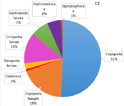
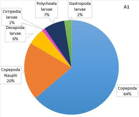
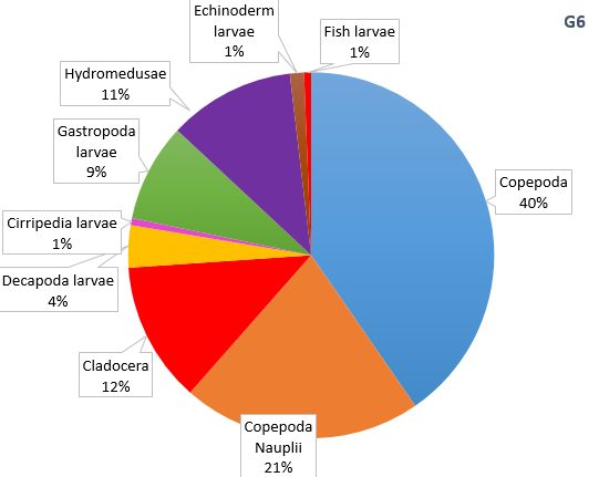
Figure 15. Zooplankton species composition at three sites along the Fal Estuary. Pie charts display identified zooplankton species to the highest taxa possible using identification catalogues. Three sample sites represent the upper estuary (A1), mid estuary (C3) and lower estuary (G6). Percentages represent the calculated species composition per ml of each individual site. Samples collected using a tow net.
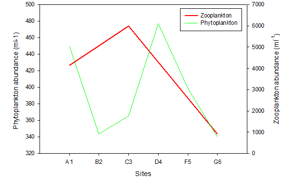
Figure 16. Total phytoplankton and zooplankton abundance at six sites along the Fal Estuary. Abundance calculated using a 1000ml sample collected from each site using a tow net. Sites range from the upper estuary (A1) to the mouth of the estuary (G6).
Discussion
Riverine water is high in silicon due to terrestrial input by weathering. Since riverine water is less dense than seawater, input of nutrients will be trapped in the upper surface layer especially if there is limited mixing . Silicon is taken up by siliceous diatoms to use in test formation. Therefore high diatom activity will result in low silicon concentrations (Fig.11). The high abundance of Chaetoceros across all stations (Fig. 13) correlates with the decline in silicon downstream (Fig. 11). Therefore the uptake of silicon by siliceous diatoms will reduce the downward flow of the nutrients. Higher nitrate levels in rivers and estuaries compared to seawater results from terrestrial and anthropogenic inputs into the estuary [19]. The decrease in nitrate down the estuary can be attributed to removal by phytoplankton, as nitrate is a vital nutrient needed for DNA production [20]. The highest phosphate levels at the head of the estuary (A1) are a result of input from increased soil disturbance and waste discharge [21]. The high levels of phytoplankton upstream will cause a decline in phosphate concentrations, as phosphate has been shown to be essential for zooplankton growth [22].
Phosphate has been shown to limit phytoplankton growth more than nitrogen [23]. An increase in constraining nutrients such as phosphate can increase phytoplankton and macroalgae growth, having a large effect on the estuarine and coastal ecosystem [21]. The large ranges on phosphate concentrations seen at sites A1 and B2 can be due to high noise levels, altering the data (Fig. 10). The phosphate levels are therefore unreliable. The residence time of a macrotidal estuary can also be a cause of the rapid loss of nutrients downstream. Strong tidal ranges see a high flux of water in and out of the estuary, flushing nutrients out, away from the riverine source before they can settle [24]. Decreasing oxygen with depth is to be expected in an estuarine body, as its input through the atmospheric boundary is preferentially used up by respiring organisms in the column but at site A1 oxygen increases with depth. This could correlate with the biological figures, that found chlorophyll and backscatter maximums at the seabed. However the minimal oxygen available at such depths suggests photosynthesis would not be available, and is likely to depict an error in the measurements. Moving from site C3 to G6 oxygen concentration decreases as oxygen is used up by the photosynthesising phytoplankton.
Optimum salinity range for brackish species is between 5 and 8, whereas total species richness in an estuarine ecosystem reaches a minimum across this range. At higher and lower salinities, marine and freshwater species will dominate respectively [13]. The data collected in the Fal Estuary reflects this pattern (Fig. 16). Research shows dinoflagellates favour stable waters and aggregate at the surface [14] The very low abundance of dinoflagellates across all sites (Fig. 13) could be a result of the scale of the tidal range, that leads to almost constant movement and hence a relatively well mixed column of water. Identification error to a species level has been found to account for considerable error [15]. Diatoms rely on increased turbulence to remain in a zone of both sufficient irradiance and nutrient availability [16]. Although the highest nutrient levels are seen in the upper estuary, the preferable salinity range downstream could be the reason for higher phytoplankton abundance at G6 (Fig. 16). Diatoms can assimilate nutrients faster than other phytoplankton, enabling them to outcompete dinoflagellates [17]. This provides further evidence for the low abundance of dinoflagellates.
The decline in phytoplankton and rise in zooplankton between sites B2 and C3 suggests a time lag in the consumption of phytoplankton by zooplankton and therefore increase in their growth rates [18]. Evidence from the ADCP transect (Fig. 7) could suggest the upstream flow in the middle of the estuary is limiting movement downstream, resulting in high zooplankton at site C3. It should be noted that the data we collected in the Fal estuary however does not show temporal variation. Hence the presence of a bloom cannot be easily determined from this data alone.