Offshore

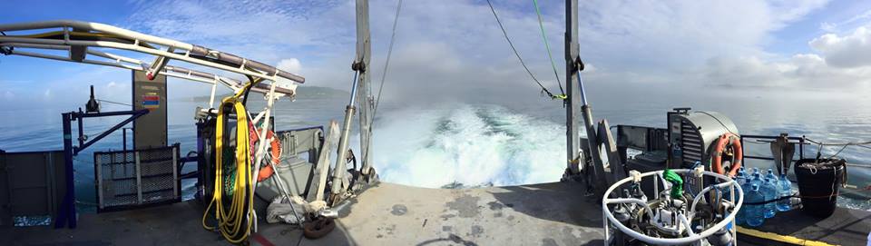
The aim of this session was to determine the structure of the water column in coastal seas, how it changes as one goes further out to sea, the drivers of these changes and how these factors affect the local planktonic communities. This was achieved through CTD and ADCP profiling, water sample collection and plankton sampling using nets.

Methods

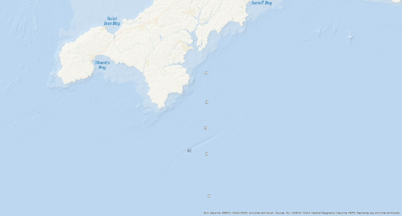
Data was taken at 5 stations, numbered 45-49. Firstly, the CTD with a rosette of 6 Niskin bottles was sent down to the bottom of the water column, giving a profile on the way down. This profile was analysed, usually with respect to temperature and chlorophyll, to determine the depth at which depth the Niskin bottles would be fired. The CTD and rosette were then raised, stopping to close the bottles where needed.

The storage method for samples was analogous to the method used on the Conway (Fal Estuary sampling); water for silicon analysis was stored in numbered plastic bottles, samples used for phosphorus and nitrogen analysis in numbered brown glass bottles, and oxygen in transparent numbered glass bottles. For chlorophyll 50ml of water was filtered through a syringe and filter paper, the filter paper was then stored in numbered tubes with 6ml of acetone and were frozen overnight. Phytoplankton samples were placed in brown glass bottles and fixed with lugol’s iodine.

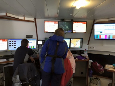
Backscatter data from the ADCP and various profiles from the CTD were used to determine where in the water column zooplankton samples should be collected. The zooplankton net was deployed down to the deeper depth of the range, pulled up to the upper limit and then, using a bronze messenger, the net was closed and brought to the surface. The zooplankton samples were stored in large labelled plastic bottles and fixed with formalin. ADCP data for flow velocity, direction and backscatter was recorded at every station and also in transit between stations.

(Back to top)

Results and Discussion

Temperature

For all stations, the same overall pattern applies; there is a significant decrease in temperature with depth from the surface to 20m depth. After this, the temperature remains level with depth. This shows a very distinct thermocline, developed due to less mixing in the upper water column from wind with the introduction of calmer weather, as well as more warming of the surface oceans with warmer weather. The thermocline coincides with the pycnocline, as temperature has a significant effect on density.

Density

All of the stations show a similar pattern; density increases slightly with depth from the surface to about 10m. After which there is a more significant increase in density with depth between 10m and 25m. From 25m to the bottom of the profile, the increase is, again, less steep. Warm water is less dense, and so will overly the cooler water. This creates stratification and a pycnocline, which can be seen on the graph as the sudden change in density. With the calmer weather coming in, there will be less mixing of the upper layer of the ocean, so the stratification will remain.

Nutrients

At Station 45, the phosphate concentration stays fairly steady from the surface to 20m, before it begins to increase with depth. Both silicon and nitrate show a much steeper increase with depth. This is the profile that would be expected of bioavailable nutrients in a depth profile. Silicon, phosphate and nitrate are all taken up by phytoplankton for various functions (e.g. silicon is used for diatom frustules, phosphate in the manufacture of ATP and nitrate for protein formation). This uptake causes each nutrient to become depleted in the surface waters. Negligible uptake occurs below the pycnocline, as phytoplankton are less inclined to congregate there due to lack of light. This causes the nutrient levels to increase beyond the pycnocline.

Station 46 shows no increase in nitrate concentration before 30m depth, when there is a very significant increase. There is a similar pattern in silicon and phosphate concentration here, however, before 30m depth, the two fluctuate more than the nitrate, and their behaviour appears to have an inverse relationship; an increase in silicon seems to encourage a decrease in phosphate. This can be said until 30m depth, at which point, there is a similar increase as seen in the nitrate.

At station 47, there is a straight increase in silicon concentration with depth, while, for phosphate and nitrate, there is a more exponential increase with depth.

The concentration of nitrate and phosphate at station 48 follow a similar pattern; from the surface to 20m depth, there is a significant decrease in concentration with depth. After this, it decreases in a slower rate. At 30m depth, there is a significant increase in concentration with depth. The concentration of silicon fluctuates strongly, with an initial significant increase with depth. At a depth of 20m, there is a significant decrease with depth. At 30m depth, it is a significant increase with depth again.

Station 49 has a similar relationship between silicon and depth as seen at station 47. Phosphate concentration initially decreases significantly with depth, with a minimum concentration at ~24m, before a significant increase to a level similar to the surface by 50m depth. The nitrate concentration does not fluctuate between the surface and ~24m depth. After this, it shows a significant increase with depth.

(Back to top)

Oxygen

Oxygen concentration decreases with depth in stations 45, 47 and 48. In station 45, oxygen concentration decreases from 250 µmol/L at the surface to 230 µmol/L at the bottom (~50m), while in station 47, oxygen concentration decreases from 270 to 240 µmol/L, and in station 48 from 310 to 260 µmol/L from surface to the bottom.

In station 46, oxygen concentration increases from 250 at the surface to 370 µmol/L in mid-depth (~25m) and then decreases to 240 µmol/L on the bottom (~60m).

In station 49, oxygen concentration increases from 250 µmol/L at the surface, to 270 µmol/L in mid-depth (~25m), and to 400 µmol/L on the bottom (~50m).

The oxygen concentration profile for stations 45, 47 and 48 decreases with depth. This can be explained by decrease in atmospheric interaction and phytoplankton and zooplankton oxygen consumption.

In stations 46 and 49, oxygen concentration increases from surface until 25 meters. This can be explained by remineralisation and decomposition of sinking organic matter. Station 46 decreases oxygen concentration from ~25m to the bottom (~60m), which can be explained by phytoplankton and zooplankton oxygen consumption. Station 49 shows an opposite trend, and keep increasing oxygen concentration from ~25m until the bottom, which can be explained by another water mass flowing under the estuary water that is enriched in oxygen.

Fluorescence

Analogous to the Chlorophyll data, fluorescence has a maximum between 20m and 30m, this will relate to the fluorescent nature of chlorophyll, which would have been the main molecule activated by the fluorometer. Between the maximum, there is not much notable activity, with significant increases at the peak. The reasons for these peaks are specified further down in the “Chlorophyll” section.

Chlorophyll

Again, between each station, there is a similar pattern. There is a chlorophyll maximum between 20m and 30m, with a steep increase and decrease with depth either side. This relates to the mass of photosynthetic phytoplankton, the main number of which is within this same range. Phytoplankton tend to congregate around the pycnocline in stratified waters, in order to benefit from nutrient rich waters below, but still remain in an area of high light intensity. Our chlorophyll maximum appeared slightly lower than the pycnocline, because the nutrient concentrations increased at a greater depth.

(Back to top)

Phytoplankton

For every station, the peak of phytoplankton is between 20-30m depth. One notable species, significantly the most dominant in 3 out of the 5 stations (45, 46, and 47), and present every vertical toe, spare two (50m at Station 45 and 55m at Station 46) is Ceratium fusus. At station 45, Ceratium furca is also significantly dominant, especially at ~20m depth, but not as high in numbers overall as C. fusus. The large numbers of C. fusus indicates a bloom. For a bloom, C. fusus needs permanent stratification, and are as such common in summer. The depth and presence of the pycnocline is important to this species (Dickson et al 1992). When looking at the density profile, distinct stratification can be seen; a clear pycnoline, which would support the idea of a C. fusus bloom. At station 48, there is a more even spread of species, but the most dominant group are the Ciliates. At station 49, the most dominant species is Dictyocha fibula, although this species is not present at the ~8m sample, where Ceratium fusus was most dominant. D. fibula is a silicoflagellate, which provides explanation for the depleted silicon in surface waters. It’s optimum growth temperature is 10°C with a salinity of 24PSU (Van Valhenbug & Norris, 1970), which is lower than what was experienced at our stations, offering explanation as to why it was not dominant at all stations. There were also large numbers of Noctiluca scintillans, but due to their large size they were mainly caught during zoplankton net trawls.

Zooplankton

For all the stations, the peak of zooplankton is around the 20m area, slightly above the peak of phytoplankton, which is to be expected as phytoplankton are a known valuable food source for zooplankton. Notable groups present in all samples are Copepoda, Cladocera, and Polychaeta larvae, with Chaetognatha and Siphonophorae appearing in almost all samples.

Cladocera and Copepoda both have a wide temperature range, so have a widespread distribution across the world. The two groups also have similar dispersal methods and interspecific niches, which is why they are both so common in all of our samples (Clifford Carl, 1940).

Larval zooplankton (such as polychaetes) are neutrally buoyant, therefore not capable of navigation, and are distributed purely by the water masses (Banse, 1986).

(Back to top)

ADCP

Station 45

At approximately 10m we observe a significant decrease in the velocity of the water column which coincides with a steep increase in the water density between 10-20m. The interaction between the two separate water masses causes friction at the boundary layer which results in a decrease in the waters velocity. Other than the reduced velocity at 10m depth the horizontal velocity remains relatively constant with time. The chlorophyll maximum at this station is present at approximately 30m depth above this depth (10-20m depth) we observe the greatest backscatter indicating a high presence of zooplankton. Our zooplankton sampling confirms this interpretation as we see the maximum number of individuals between 10-20m (~2900 per m3). These boundaries remain constant with time.

Station 46

The chlorophyll maximum and the thermocline are both present at approximately 30m depth we observe the greatest backscatter above and below this depth indicating significant zooplankton population on both sides with the greater being above the thermocline. The zooplankton sampling indicated similar results with the greatest numbers recoded between 20-30m (~2900 per m3) while a still significant presence between 30-45m (~700 per m3). Across the 47 minute measurement period we observe a decrease in the velocity of the water column caused by the ebbing of the low tide

Station 47

Very little back scatter is observed throughout the water column indicating a very low presence of zooplankton. The maximum velocities observed at the thermocline indicate the breaking of internal waves and the resulting forward momentum being transferred to the thermocline boundary layer causing increased velocities within the thermocline. This requires a strong thermocline to be present otherwise the forward momentum isn’t contained and is dispersed throughout the water column.

Station 48

The chlorophyll maximum and the thermocline are both present at approximately 20m depth, similar to the results of station 46 significant zooplankton populations are located above and below this depth (between 10-35m). Higher number of zooplankton observed at station 48 than previous stations (~3600 per m3). We observe an increase in the waters columns velocity across the 31 minute sample period, this increase is due to the approaching high tide at ~13:10 UTC with the greatest increase is observed bellow 10m depth.

Station 49

The chlorophyll maximum and the deepest instance of the backscatter peak coincide at approximately 25m this indicates that the greatest density of zooplankton is located above the chlorophyll maximum. A large protrusion (~35m in height) from the bathymetry resulted in some localised interference nevertheless the depth of the zooplankton maximum remains constant with time. We observe a general increase in the velocity of the water column with time, however the speed of the surface waters (0-10m depth) remain a relatively high constant.

Richardson numbers

Although there is significant fluctuation, in general, the flow is turbulent at the surface and the bottom of the water column and the flow is laminar in between, in the general water column. This is to be expected, as there will be turbulence where a boundary lies i.e. the seafloor and the air/sea interface. At station 49, there is a point, below 20m depth, where the flow is turbulent again. This can be explained by the presence of the thermocline, which acts as another boundary layer. There are a few points at the other stations where this change of flow is present, however these are not in the same areas as the thermocline, so cannot be explained by this.

References

Dickson, R.R., Colebrook, J.M., Svendsen E., 1992. Recent changes in the summer plankton of the North Sea. ICES Marine Science Symposia. 125. pp. 232-242

Banse, K., 1986. Vertical distribution and horizontal transport of planktonic larvae of echinoderms and benthic polychaetes in an open coastal sea. Bulletin of Marine Science. 39:2. pp. 12-17(14)

Clifford Carl, G., 1940. The Distribution of Some Cladocera and Free-Living Copepoda in British Columbia. Ecological Monographs. 10:1. pp. 55-110.

Date: 29.06.15

Time: 08:24 (UTC)

Location:

Station 45 - 50° 05, 605’ N

4° 51, 564’ W

Station 49 - 39° 41, 979’ N

4° 51, 154’ W

Low tide: 10:13

High tide: 16:10

Cloud cover: Varied from 6/8 - 8/8

Sea state: Varied from 1/10 - 2/10