
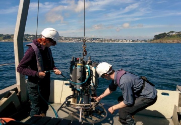
The aim of this trip was to determine how the structure of the water column varies down the estuary, particularly with respect to stratification and mixing and its subsequent effect on nutrient and plankton distribution. This was achieved through CTD and ADCP profiling, Niskin bottle sampling and zooplankton net trawls.
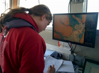
Data was taken at 4 stations numbered 24-
From the samples collected by the Niskin bottles, water was stored in various bottles for analysis at the lab the following day. Water for silicon analysis was stored in numbered plastic bottles, water samples for phosphate and nitrate analysis were stored together in the same numbered dark glass bottles. Oxygen water samples were stored in separate transparent numbered glass bottles. 50ml of water from each bottle was filtered through a syringe for chlorophyll. The filters were stored in separate numbered tubes, filled with 6ml of acetone. These samples were frozen overnight for lab analysis the following day.
An ADCP transect was also carried out at every station. The start and end latitude and longitude were recorded. Each transect measured currents, area, and flow velocity across the river. This allowed for the calculation of river flushing time at each area.
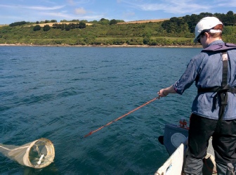
At 2 of the 4 stations, Zooplankton and Phytoplankton samples were taken. The phytoplankton samples came directly from water in the Niskin bottles, and were placed in brown glass bottles with lugol iodine. The zooplankton samples were collected via a horizontal trawl using a net with a mesh size of 200µm and a diameter of 0.6m. A flow meter was attached at the mouth of the net in order to calculate the total amount of water sampled. Each tow lasted exactly 5 minutes. Samples were fixed with formalin and stored in large plastic bottles labelled B and C.
Chlorophyll
In most of the stations, chlorophyll concentration increases with depth until a maximum concentration, and then decreases until the bottom.
Station 16 shows a surface chlorophyll concentration of 5 µg/L, a maximum of 12 µg/L around 2 meters deep, and then decrease concentration until the bottom with some variation. The same pattern was observed in stations 17 and 18, with surface values of 8 and 7 µg/L, maximum of 9 and 11 µg/L at 2 and 4 meters deep, respectively, and then concentration decrease until the bottom. Chlorophyll concentration in station 20 varies until 5 meters deep, showing a maximum of 9 µg/L. Station 20 showed the lowest chlorophyll concentration values, with a maximum of 1.9 µg/L at 2 meters deep. Surface chlorophyll concentration in station 21 was 5 µg/L, increasing to 7 µg/L (2 meters deep), and then decreases until the bottom, but with a minimum around 4 meters. Stations 23, 24, 26, 27 and 28 showed the same pattern of a maximum, and then decrease until the bottom, but without much variation. Surface concentrations for stations 23, 24, 26, 27 and 28 was respectively 2, 2, 0.5, 1.3 and, 0.3 µg/L, maximum of 4.8, 4.5, 2.3, 2.7 and 2.1 µg/L, respectively, at depth of 8, 8, 10, 15 and 14 meters.
In station 28 was observed the lowest chlorophyll concentration value of 0.3 µg/L, and highest in stations 17 and 18, of 9 µg/L. Chlorophyll concentration maximum of 12 µg/L was observed in station 16, at 2 meters deep.
Dissolved Oxygen
Dissolved oxygen patterns was very similar in most stations, showing a maximum in surface, then slightly decreases with depth until chlorophyll maximum, and then decreases until the bottom. This pattern was observed in stations 16, 17, 18, 19, 20, 21, 23, 24 and 26, with a surface concentration of 17, 11, 10, 9, 1.8, 7, 4.8, 4.5 and 2.1 µg/L, respectively.
In station 27, dissolved oxygen concentration decreases constantly until the bottom, showing 2.7 µg/L as surface concentration. Station 28 showed a different pattern, dissolved oxygen concentration increases from surface (1.7 µg/L) until a maximum at 10 meters (2.3 µg/L) and then decreases until the bottom.
Nutrient Distribution
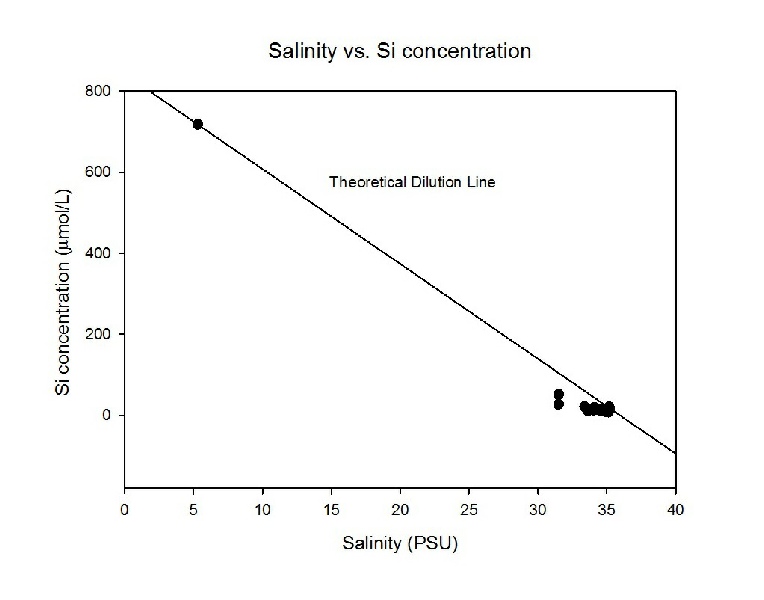
Silicon
Along the transect, there was very little salinity variation. There is a bit of a dip in silicon concentration below the theoretical dilution line.
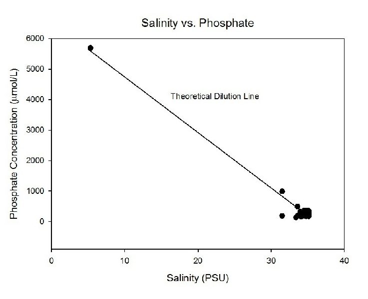
Phosphate
There is again not much variation in salinity, making the data points appear as a cluster at the high salinity end, with three points scattered at a salinity of about 30PSU to 33 PSU. Two of these points appear slightly about the TDL, with one point appearing quite a way below the TDL.
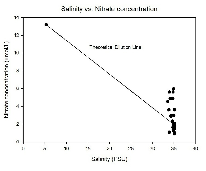
Nitrate
The data points are very clearly scattered around the theoretical dilution line, more so that with silicon or phosphate. A few points appear a long way above the TDL, with a cluster of points also appearing below the TDL.
All nutrients have their highest concentrations at the riverine endmember.
Oxygen
Dissolved oxygen concentration is higher in surface for all stations, and decrease
with depth because of its consumption by phytoplankton and zooplankton, and decrease
of atmospheric interaction. A slight decrease of dissolved oxygen concentration occurs
until it reaches the maximum chlorophyll concentration depth, mostly because of decrease
in atmospheric interaction. Then dissolved oxygen decreases more rapidly with depth
because of phytoplankton and zooplankton consumption. Chlorophyll concentration increases
from surface until reaches a maximum and then decreases with depth. It occurs because
in surface there is enough light for phytoplankton growth, but nutrients are limiting
factors for surface caused by halocline and thermocline that do not allow nutrients
to come to the surface. In mid-
Nutrient Distribution
The fact that the samples taken had salinities very close together makes it very
hard to work out whether each nutrient is conservative or non-
The dip below the TDL for silicon may indicate that it is being depleted, but more data points across a range of salinities are needed to make this judgement.
Phosphate is likely to be conservative, as only a little scatter occurs both above and below the TDL. Again, more data points are needed to make a judgement.
Nitrate is the most likely nutrient to show non-
Temperature Salinity Profiles
The overlying water is the riverine input, which is fresher and warmer. The cooler, more saline water mass lies below, and is the tidal input. Cool saline water is denser than warmer fresh water, which creates stratification within the estuary. The fresh water at the surface will be warmed by solar radiation, accounting for the thermocline. It is clear from our T/S profiles that the Fal Estuary is highly stratified.
The increase in thermocline/halocline depth with movement towards the estuary mouth reflects the fact that we were moving into deeper water. The increase in average salinity towards the mouth of the estuary reflects the diminishing river input. The fact that the change is so small, despite covering a large area of estuary is due to the fact that the freshwater input in the Fal Estuary is low (Brigden, 2005), with the estuary being almost fully marine (Deeble & Stone, 1985). This creates a well mixed estuary.
Transects of the Fal Estuary were taken in the upper and lower estuary. The upper estuary transects were taken during an incoming tide and therefore show an overall northern flow while the lower estuary transects were taken after high tide as so show a southerly flow. The total discharge of water through the transects is effected by both the tide state and how far the transect is down the estuary. The faster the tidal current the higher the total Q at a transect. The closer a transect is to the mouth of the estuary the greater the total Q as it has to empty a greater area of water each tidal cycle. Figure 1 shows the locations of all transects.
Station 16
Greater velocity is seen on the west bank of the channel. This may be due to the
shape of the cross-
Date: 25.06.15
Time: 12:15 (UTC)
Location: Start: 50° 12, 203’ N
5° 02, 419’ W
Finish: 50° 08,723’ N
5° 01, 422’ W
High tide: 11:05 4.1m
Low tide: 17:35 1.8m
Cloud cover: 2/8
Sea state: 1/10
Disclaimer-
Falmouth 2015 Group

Oxygen and chlorophyll profiles
TS Profiles
ADCP Transects
Track plots
Station 17
There is a greater velocity on the east bank and particularly at the surface. At this point in the estuary the water is flowing around a meander with the east bank on the outside. As water flows fastest on the outside of a meander this explains the greater velocity here. Relatively high speeds are seen as the incoming tidal current is still strong. Figures 4 and 5 show the Velocity Magnitude and Track Plots for Station 17.
Station 20
There is an overall reduction in flow velocity here as at this time the incoming tidal current is weakening as it approaches high tide. There is northward flow on the west bank of the estuary and a slight southern flow on the east bank. The reason for this may be that there is a confluence just north of this station which may contribute a southern flow that can cancel out the weak tidal flow. Figures 6 and 7 show the Velocity Magnitude and Track Plots for Station 20.
Station 21
Overall velocity is much lower due to the imminent high tide. The channel at this station is straight. There is therefore less interference for meanders. This results in the fastest flow moving up the centre of the channel. Figures 8 and 9 show the Velocity Magnitude and Track Plots for Station 21.
Station 25
This transect was taken some nearly 2 hours after high tide which has resulted in a faster southerly flow. This transect is at the mouth to the expanded part of the estuary basin. This may also explain the sudden increase in flow as the estuary water suddenly has to fill a much larger area. Figures 10 and 11 show the Velocity Magnitude and Track Plots for Station 25.As the Richardson Number defines that flows with Ri>1 are laminar and Ri<0.25 are turbulent, Station 25 presents a turbulent flux on the surface, followed by a laminar that gets turbulent again from 6 to 10m depth and from 11m to the bottom it gets laminar and stable. This turbulence in the middle of the water column might be caused by the mixing between river water and seawater.
Station 26
At this time the outgoing tidal current is speeding up which results in an increase in velocity. There are slightly higher velocities seen in the main channel at the bed and near the surface with slower currents at intermediate depths. This slower section coincides with the thermocline and halocline which is where two bodies of water with different temperatures and salinities are moving past each other which may create shear stress and slows the flow of water. Greater velocity in the main channel seems to be slightly more on the west bank. A possible reason for this may be that the outgoing tidal current is being pushed to the right by Coriolis force. Figures 12 and 13 show the Velocity Magnitude and Track Plots for Station 26. For station 26 the CTD data was dubious as it showed salinity 36 in the estuary, giving anomalous density results and therefore was not used. For that reason, the Richardson Number profile couldn’t be completed. However, it showed a turbulent flow at surface that got laminar from 5 to 6m, reasonably similar to station 25.
Station 27
This transect was taken when the outgoing tidal current is at its strongest. However, as the channel is much wider than before the water does not need to flow as quickly. There is a slightly faster flow on the east bank of the channel. This may be due to the estuary bending slightly to the west, meaning the water on the outside of the bend (east side) will flow slightly faster. Figures 14 and 15 show the Velocity Magnitude and Track Plots for Station 27. For station 27, from 7m to 9.5m the flow is laminar and gets turbulent past 10m depth. Comparing stations 25, 26 and 27 (station 25 was at the end of the upper estuary at around midday and station 28 was already at the middle of the lower estuary at around 14:30), and giving that the high tide time was at 11:05 losing strength by the time station 27 started to be sampled, the influence of the seawater at surface decreased and the surface flow started to get less turbulent. The turbulence at the bottom might be due a shear stress.
Station 28
Outgoing tidal currents are still strong at this time resulting in a fast southerly flow. The greatest velocities are seen on the west side, particularly at the surface, of the estuary which may be due to the Coriolis force pushing the southward current to the right. The faster flow at the surface may be due to the lack of friction with the banks at these points in the estuary. Figures 16 and 17 show the Velocity Magnitude and Track Plots for Station 28. Station 28 shows more turbulence within the water column which might be explained by the location of this station (black rock), which is at the mouth of the estuary, and therefore influenced by the open ocean turbulence.
Brigden, A., 2005. Dredging Protocol: Baseline Document Fal and Helford Estuaries. Carrick District Council. [online] Available at: <www.portoftruro.co.uk/files/downloads/2011/07/dredging_protocol.pdf> [Accessed 02/07/2015]
Langston, W. J., et. al., 2003. Site Characterisation of the South West European Marine Sites: Fal and Helford cSAC. [online] Available at: <www.mba.ac.uk/nmbl/publications/charpub/pdf/Fal_Helford.pdf.> [Accessed 02/07/2015]
Deeble, M., Stone, V., 1985. A port that could threaten marine life in England’s
Fal Estuary. Oryx. 19:02 pp. 74-
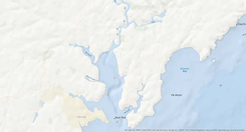
Station Locations for estuary work
Ri number plots
| Aims |
| Methods |
| Results and Discussion |
| References |
| Benthic Habitat Map |
| Cameras |
| Aims |
| Methods |
| Results |
| Discussion |
| Aims |
| Methods |
| Results |
| Discussion |
| References |
| Aims |
| Methods |
| Results and Discussion |
| References |
| Temperature and Density |
| Nutrients and Oxygen |
| Chlorophyll and Fluorescence |
| Plankton |
| ADCP |