Overview

An investigation on board the RV Callista, using CTD equipment, niskin bottle rosette sampling and phytoplankton nets designed to collect data to show the changes that occur over half a tidal cycle, at a site north of the Manacles.
The temperature, salinity, chlorophyll  levels and depth were measured and recorded using the CTD, then qdrch were to identify the thermocline and chlorophyll maximums within the water column, and to see how these structures changed with the tidal cycle, between two stations, one close to the coast and one further out to sea.
The water samples were used to work out the silicate, phosphate, dissolved oxygen, nitrate and chlorophyll levels in the water at different depths depending on the water structure at each site.
The site was selected based upon previous group’s data and on the weather conditions of that particular day.

Meta data

Date: 27/06/2014

Time: 07:15-17:15  UTC

Location: NE of The Manacles

Weather: 8/8 cloud cover, light to heavy rain, reasonable winds

High tide: 05:20  4.6m

Low Tide: 12:04  0.9m

Methods

Sampling

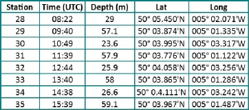
Samples were taken at two locations situated slightly north of The Manacles (figure 1); a set of rocks off the Lizard peninsula and a popular spot for scuba diving due to the number of shipwrecks nearby. Due to weather conditions we were forced to remain close to the shore. However, this enabled us to create a time series around the Manacles as the tide changed throughout the day.

Sampling methods included using a CTD rosette system with Niskin bottles attached to create a vertical profile of the water column. Samples from the bottles were used to calculate % Oxygen saturation and chlorophyll, nitrate, silicate and phosphate concentration. Vertical nets with a mesh of 200µm and open diameter of 62cm were used to collect plankton. The Acoustic Doppler Current Profiler (ADCP) and a Seabird thermosalinograph recorded data continuously throughout voyage.

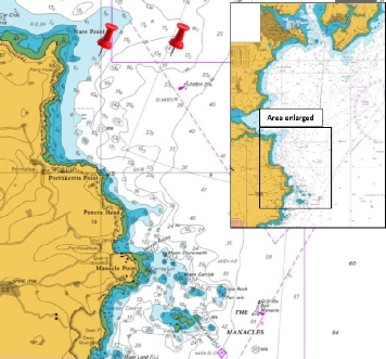
Figure 1. Sea chart of the area where samples were taken. The two locations sampled are indicated by pins. These location were revisited at one hour intervals.

CTD: The CTD rosette system was deployed to the surface using an A-frame and ropes to control the swing in the rough sea. Data acquisition was initiated, the CTD was lowered to almost bottom depth and the vertical profile of temperature, salinity and fluorescence was reviewed. Following this the CTD was raised and niskin bottles fired remotely at depths where the profile seemed interesting or unusual, for example, at the thermocline or deep chlorophyll maximum. Surface and bottom samples were taken at each station. Once back on board, water was extracted from the niskin bottles for sampling.

Secchi disk: A Secchi disk depth reading was taken at each station to estimate the attenuation of light through the surface water.

Chemistry

Oxygen: Filled a glass bottle of approx. 125ml from the niskin bottle, taking care to eradicate all bubbles. Then 1ml of manganous chloride (removes oxygen from solution forming a precipitate) and 1ml of alkaline iodide (to stain the precipitate) were added to the sample, which was then stoppered and gently shaken.

Nutrients: Sub-samples of the Niskin bottles were taken from each depth. 50ml was filtered into three bottles for analysis in the lab (one for silicon, one for phosphate and nitrate). 0.7µm glass fibre filters were used and replaced each time. The used filters were placed in acetone for analysis of chlorophyll.  

Biology

Phytoplankton: 100 ml of water from the plankton net were added to a solution of lugols iodine and left overnight to allow the plankton to bind to the iodine. After allowing them to sink, the top 90ml of excess solution was removed and the remaining 10ml used for observation under a light microscope. 1ml was analysed in a sedgewick-rafter chamber.

Zooplankton: Some samples from the plankton were separated and 40% formalin-sucrose solution was added to them before being left overnight. In the lab the following day the contents of samples were analysed under a microscope using a Bogorov Chamber.

Laboratory

Nitrate: Using a peristaltic pump a NO3 carrier stream of ammonium and sodium chloride (which mimics sea water) is drawn up with 2 reagents: 0.1% N.E.D.H (Naphthylethylenediamine dihydrochloride) and 1% Sulphanilamide. This is mixed with a fixed amount of nitrate sample and injected into the system once the nitrate has been reduced to nitrite via a copperised cadmium column. The reagents react with nitrite to form a pink azo-dye; the more nitrate/nitrite there is, the stronger the pink azo-dye will be. A strong dye will give a higher reading when it is passed through the UV spectrometer.

N.B. All sample were re-filtered in the lab to account for errors in filtering in the field.

Silicon: Standards were prepared by diluting solutions 25 times with 5ml of MQ water. 6 standards were made to construct a calibration curve of absorbance against concentration. 5ml from samples, blanks and replicates were taken, 2ml of Molybdate reagent added and left to stand for 10 minutes. 3ml of a mixing reducing reagent is then added and left to stand for 2 hours. Absorbance can then be measured using a spectrophotometer at 810nm and true concentration calculated from the calibration curve.

Phosphate: Standards were prepared freshly due to the low concentration, which can decrease at an unpredictable rate. 1ml standard stock solution was diluted 400 fold with MQ water. This is then used to make known standards of 0.15, 0.3, 0.75, 1.5, 3.0 and 6.0 µmol P/L concentrations. When absorbance of samples was measured in the spectrometer at 882nm they could be calibrated to the absorbance of the known standards.

Chlorophyll: The samples of filters in acetone were transferred to a vial and analysed in a fluorometer. Values were recorded after a calculation was made to convert the values to µg chlorophyll/L of seawater.

Oxygen: The Winkler method was used to determine dissolved oxygen concentration. 1ml of sulphuric acid was added to the samples in order to oxidise iodine ions to iodine and break down the precipitate. The solution was titrated until the potentiometric recorder ceased to rise in value. Volume of sodium thiosulphate was then used to calculate the dissolved oxygen concentration as the two values are proportionate.

CTD

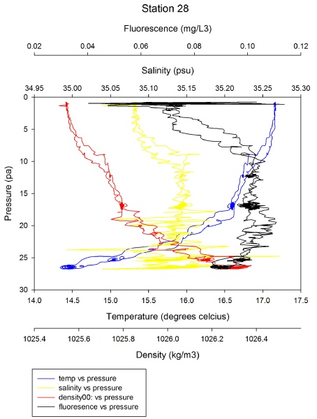
Station 28: The temperature was highest (17.2°C) at the surface, it then decreased gradually in the first 20pa. However, after this point there is a rapid temperature decrease to 14.3°C at the bottom of the water column, which is the lowest temperature recorded.  Density appeared to be inversely proportional to temperature; it was low at the surface (1025.55 kg/m3) and highest at depth (1026.35 kg/m3). Fluorescence was lowest at the surface (0.07mg/L3), then increased with depth reaching a maximum (0.115mg/L3) at a pressure of 20pa. Fluorescence then decreased down to (0.09mg/L3) at the bottom of the profile. Salinity was low at the surface (35.08) and then increased with depth until approximately 9pa where it reached a maximum of 35.15. After 9pa the salinity remained uniform down to the bottom of the water column

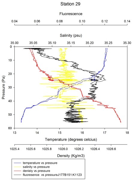
Station 29: Temperature was similar to station 28. The maxima was at the surface (17.1°C), with little decrease down to 20pa. At 20pa temperature decreased rapidly to 13.4°C at 45pa. The temperature then remained fairly steady until the bottom at 56pa. Density, as expected, was inversely proportional to temperature and, therefore was low at the surface (1025.6 kg/m3). Density then increased rapidly in the intermediate depths until 45pa where it increased much more gradually to the bottom of the profile.There was a very pronounced deep chlorophyll maximum at station 29 (0.118 mg/L3 at 22pa) and very low fluorescence at the surface (0.06 mg/L3). After this point the fluorescence begins to decrease, reaching (0.09 mg/L3) at the deepest point in the profile. Salinity was fairly constant throughout the water column with a slight increase relating to the fluorescence maximum at 22pa in the middle of the water column. There is also a noticeable increase near the bottom of the profile, possibly due to turbulent mixing, causing the re-suspension of sediment.

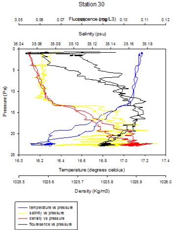
Station 30: Temperature was again high at the surface (17.1°C) then decreased gradually until a pressure of 13 pa. Temperature then decreased more quickly, reaching a minimum (16.2°C) at the deepest point of 23pa. It should be noted that the water here was fairly shallow resulting in a low range in temperature from surface to bottom. Density was also inversely proportional at this station, with the lowest density (1025.5kg/m3) at the surface and the greatest density (1025.9 kg/m3) at the deepest point. There was a sharp increase in density in the middle water column relating to the rapid decrease in temperature.Fluorescence was low in surface waters, however there was some significant variation between the down and up cast of the CTD, especially in the shallow portion of the profile. The fluorescence maximum (0.11 mg/L3) is around 13pa which relates to the thermocline. Salinity had a more pronounced variation at this station, with the lowest (35.07) at the surface, which then remained constant to around 12pa. A rapid increase in salinity then increased in the middle of the water column, reaching higher values at a similar depth to the fluorescence maximum. The maximum salinity (35.15) was at roughly 20pa with a slight decrease occurring after this depth until the bottom of the profile. There was large spiking in the graph at the bottom of the profile, likely due to the CTD being held at the bottom in order to fire a Niskin bottle.

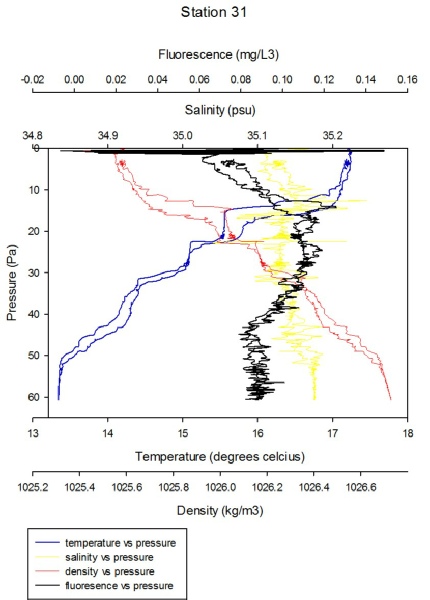
Station 31: Temperature was at its maximum at the surface (17.2°C), with a quite pronounced thermocline between 10-20pa where the temperature rapidly decreased to (15.5°C). The temperature then continued to decrease reaching its minimum (13.3°C) at the deepest point of the profile where pressure was 60pa. Density again followed temperature inversely, with the lowest density (1025.5 kg/m3) at the surface and the highest density (1026.8 kg/m3) at the very deepest point of the profile, 60pa. Density was also proportional to salinity, with more saline waters having a higher density than less saline ones.Fluorescence varies hugely at the surface, possibly due to the extended period of time spent at the surface. However an average at the surface represents the lowest fluorescence (0.07 mg/L3). Fluorescence was then at its maximum (0.11 mg/L3) between a pressure of 15-30pa, the middle of the water column, representing a deep chlorophyll maximum. There was then a decrease in fluorescence to (0.08 mg/L3) at 40pa, thereafter the fluorescence remained steady down to the bottom of the water column.Salinity was lowest at the surface (35.11), however there was little change in salinity throughout the water column until a pressure of 50pa where salinity increased slightly to (35.18).

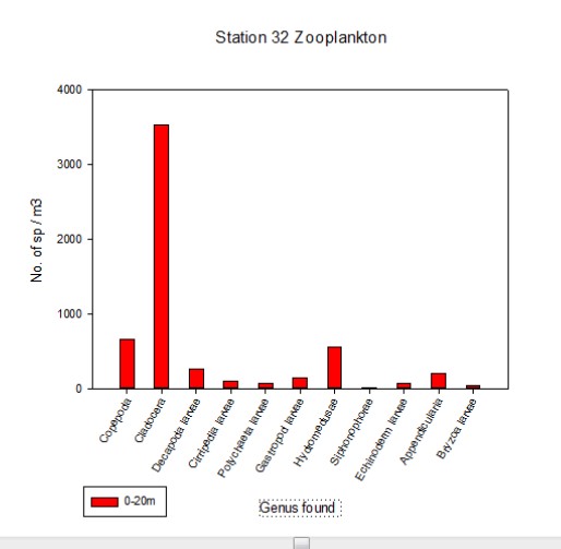
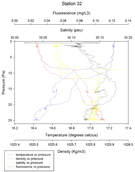
Station 32: Temperature was again the maximum at the surface (17.2 °C) remaining constant until 7pa where it began to decrease rapidly to (16.7°C) at around 15pa. There was quite a difference in temperature between the up and down cast of the CTD in the middle water column, so an average is required for the most accurate temperature. There was then a more gradual decrease in temperature until the bottom, 25pa, where the temperature reaches its minimum (16.4°C).Density was low at the surface (1025.5 kg/m3) and increased inversely with temperature. At around 15pa there was a rapid increase in density to (1025.7 kg/m3). As depth increases after this point, the density increased at a slower rate than before until a maximum of (1025.8 kg/m3) at 25pa, the deepest point in the profile.Fluorescence was lowest at the surface (0.08 mg/L3) and increased in the middle water column to a maximum of (0.13 mg/L3) at 15pa. The fluorescence then decreased to (0.09 mg/L3) at the bottom of the water column where pressure was 25pa.Salinity was lowest at the surface (35.08) remaining constant until a pressure of around 10pa at which point there was an increase of salinity to the maximum (35.15) for the water column. The salinity then remained fairly constant for the remainder of the water column, only decreasing a very small amount thereafter.

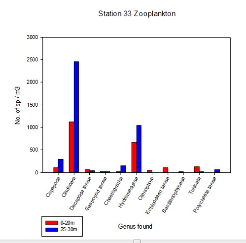
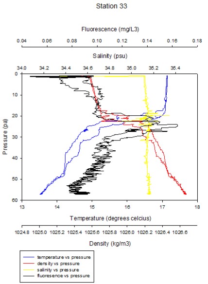
Station 33: Temperature was at a maximum (17.2°C) at the surface, and remained constant in the surface layer until around 18pa where there was a sudden drop in temperature down to around (14.7°C) at 25pa. The temperature then continued to decrease with depth at a slower rate, reached a minimum of (13.4°C) at the bottom of the profile with a pressure of 57pa.Density was at its lowest (1025.6 kg/m3) and again varied inversely proportionally with temperature. So in the middle water column it increased rapidly and reached a maximum (1026.7 kg/m3) at the deepest point.Flourescence was lowest at surface (0.07 mg/L3) and increased to a very pronounced maximum (0.15 mg/L3) in the middle of the water column, which was the highest reading out of all the stations. It then decreased again to (0.09 mg/L3) at the deepest point, 57 pa. Salinity remained very constant throughout the water column at around (35.1).

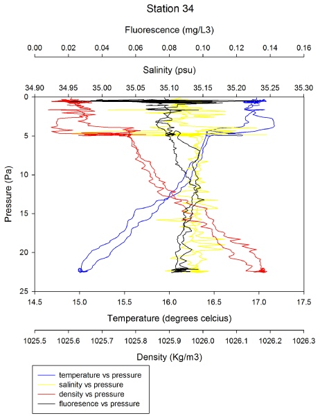
Station 34: Temperature was highest (16.9°C) at the surface, which was actually lower compared to other stations. There then appears to have been a very shallow thermocline at a pressure of 5pa, at this point temperature decreased to (16.3°C). Temperature then decreased steadily to (15°C) at the deepest point of the profile, 23pa.Density showed a minimum (1025.58 kg/m3) at the surface, which then showed an inverse pattern to temperature, and increased rapidly to (1027.50 kg/m3) at 5pa. Density then increased more steadily to a maximum (1026.18 kg/m3) at depth.Fluorescence varied wildly at the very surface, most likely due to the CTD remaining at this depth for a longer period of time. There is little variation at depth and fluorescence remained fairly constant throughout the water column ranging from (0.08 mg/L3)  at the surface, to  (0.10 mg/L3) in the middle of the water column and then down again to (0.09 mg/L3) at the deepest point.Salinity showed large spikes throughout the water column, being the lowest (35.10) at the surface and then increased to a maximum of (35.14) in the mid water column, before it slightly decreased again to (35.13) at the bottom of the profile.

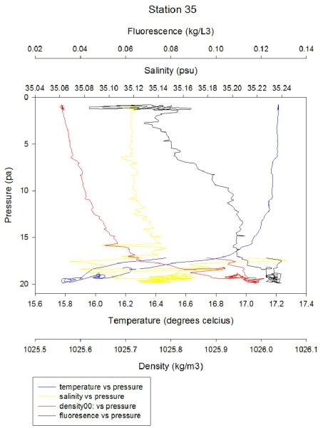
Station 35: NOTE: only a down cast CTD was taken here as the vessels power cells failed during deployment, meaning an up cast could not be taken. The downcast did not reach the bottom and therefor is not representative of the whole water column.Temperature was highest (17.2°C) at the surface, which was consistent with other stations for surface temp erature. It then stayed quite constant until 15pa where it decreased sharply reaching its minimum (15.8°) at 20pa, the bottom of the profile. Density showed an inverse pattern to temperature, with a minimum (1025.59 kg/m3) at the surface, followed by an increase to a maximum (1025.97 kg/m3) at the bottom of the profile. Fluorescence was lowest (0.065 kg/L3) at the surface and then increased with depth. However there was not such a pronounced maximum in the middle water column, possibly because there was only the down cast taken. The fluorescence maximum (0.125) is actually at the deepest part of the profile. Salinity remained constant with depth, starting at (35.12) at the surface and only increased to (35.13) at depth. There were many spikes present at depth due to the prolonged period of time the CTD spent at the bottom due to a temporary lack of power to the winch.

Analysis

Temperature was highest at the surface which is expected in a partially mixed water column, the surface waters are heated by the sun and the insufficient mixing means that warm water is not mixed to depth. Density was inversely proportional to temperature, this inverse relationship is due to decreasing temperature causing a decrease in volume due to thermal contraction. As density is proportional to volume, a decreased volume means a greater density according to . Fluorescence relates to the amount of phytoplankton present, so it is affected by nutrient availability as well as light, and therefor depth. There was a large variation in fluorescence at the surface of most stations due to the CTD rosette remaining here for a longer period of time compared with the other depths. If the variation is averaged out then the surface fluorescence is the lowest at all stations, most likely due to nutrients being a limiting factor. It can be noted that there was a fluorescence maximum in the mid water column; here the conditions will be ideal for phytoplankton growth with enough light and nutrients available. After this depth light then becomes the limiting factor meaning that the fluorescence decreased again. Salinity appears to vary wildly, this is due to being calculated from conductivity and temperature, the sensor which measures temperature takes a significant period of time to change to the correct temperature, whereas the conductivity sensor registers a change almost instantly. Although there is a lot of spiking there is still distinct salinity changes with pressure (depth). In general salinity increased in the mid water column, this may represent the increased nutrients available for phytoplankton, thus explaining the increased fluorescence in the mid water column. There was nutrient depletion in the upper water column and therefor lower salinities were present here.

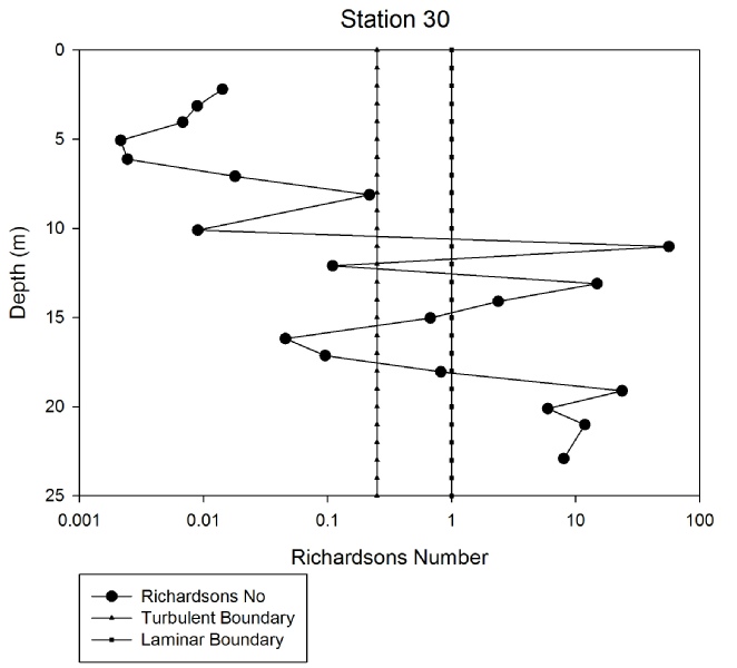
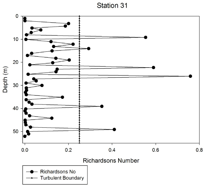
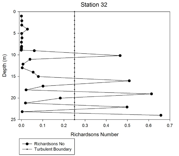
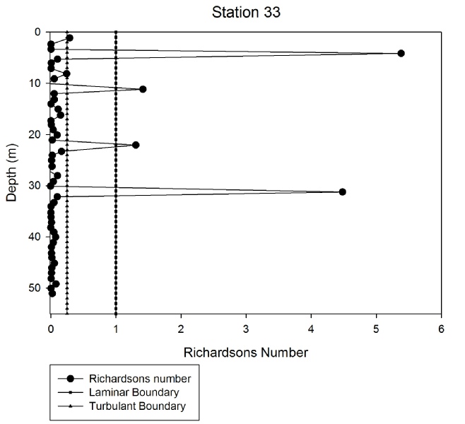
Richardson’s Number

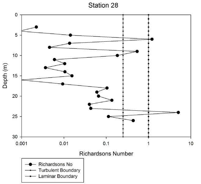
Station 28: At 6m and 9m the water column crosses the laminar boundary, apart from these depths the water column is turbulent, creating shear waves along the interface of the two water bodies which becomes unstable (1), until 25m where it again crosses the laminar boundary.

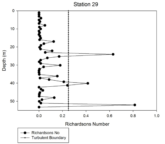
Station 29: Most of the water column at station 29 is turbulent, which induces mixing, apart from three depths (25, 39 and 53m) where the Ri number crosses the turbulent boundary into the intermediate phase but does not reach above 1; therefore flow does not become laminar and has constant mixing.

Station 30: Between 0-10m flow is below 0.25 and is turbulent, suggesting an unstable water body (1). Below this depth the water column becomes laminar before changing intermittently between turbulent and laminar flow, until below 20m where flow becomes consistently laminar and therefore likely to be less mixed.

Station 31: At most depths of station 31 the water column is turbulent apart from a few depths throughout the water colour where flow crosses to the intermediate phase. This would suggest that the water column at this station is mainly well mixed.

Station 32: Between 0 – 10m flow is turbulent and the water is well mixed, at 10m the Richardson’s number crosses the turbulent boundary but does not increase sufficiently to induce laminar flow and a stable water column. This trend continues with the water flow fluctuating around the turbulent boundary until the maximum depth of 24m; the water column never reaches laminar flow with a stable water column.

Station 33: The water column at station 33 is mostly turbulent and well mixed down to the maximum depth of 53m, excluding four depths (5, 11, 23 and 31m), where the water column reaches laminar flow and mixing between the layers at these depths ceases.  

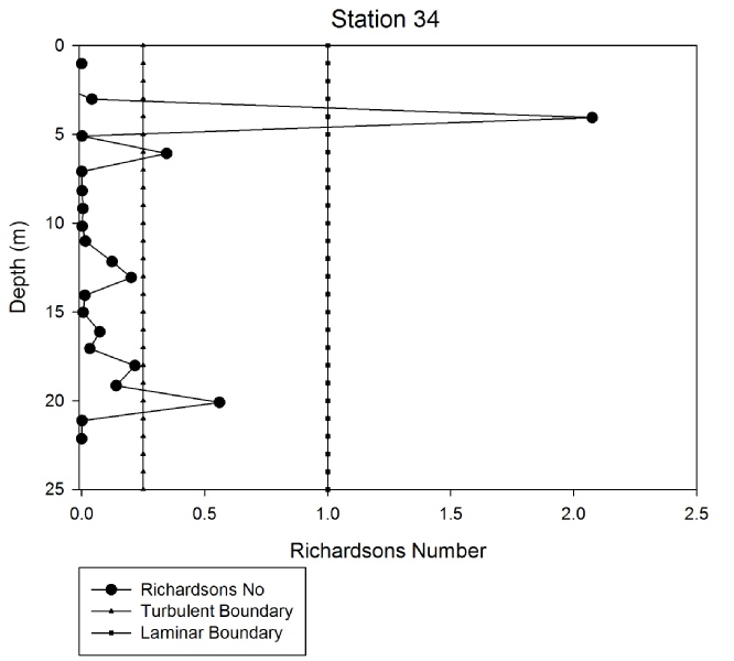
Station 34: Laminar flow is only reached at one point throughout the water column of station 34, suggesting only one point of stability. The rest of the water column represents turbulent flow and a well-mixed water column, excluding depths of 6m and 20m, where the flow crosses into the intermediate phase.

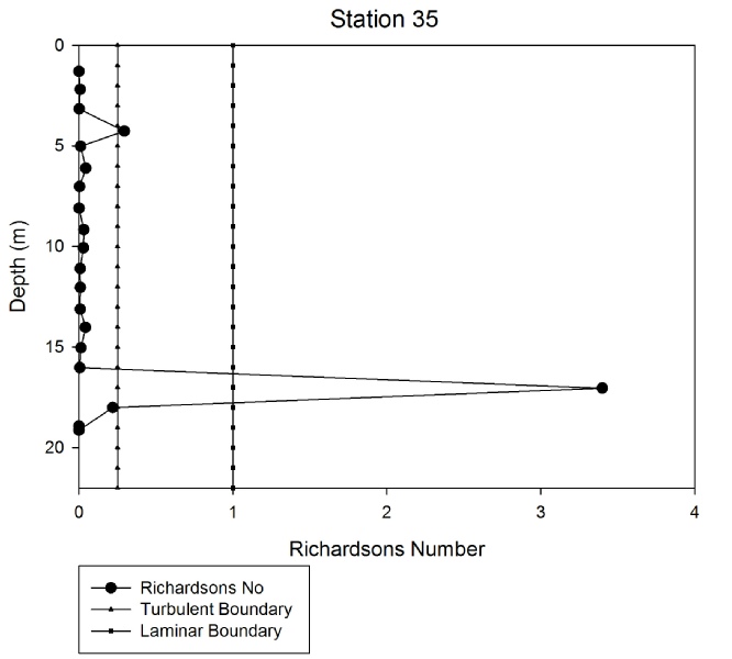
Station 35: The water column at station 35 is turbulent and well mixed throughout the water column, apart from 17m where flow becomes laminar and stable.

Results

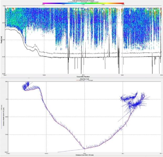
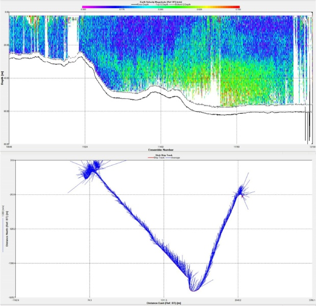
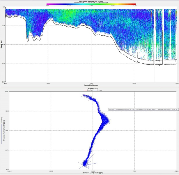
ADCP

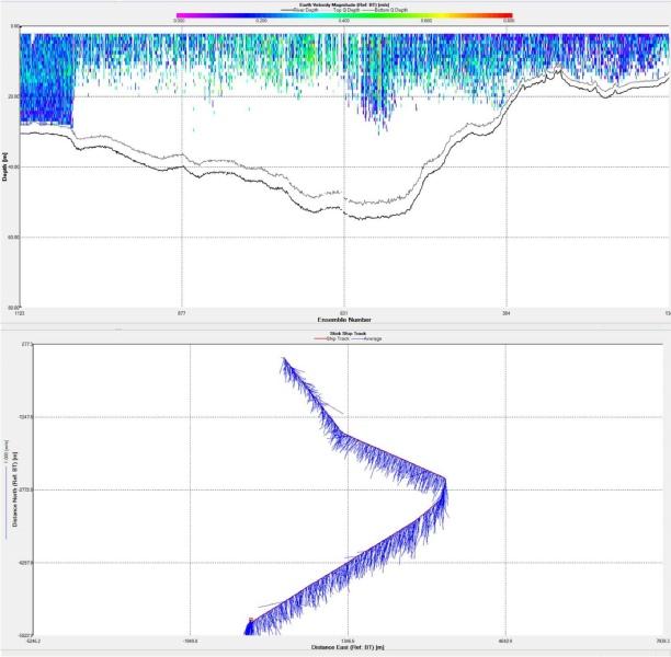
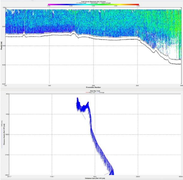
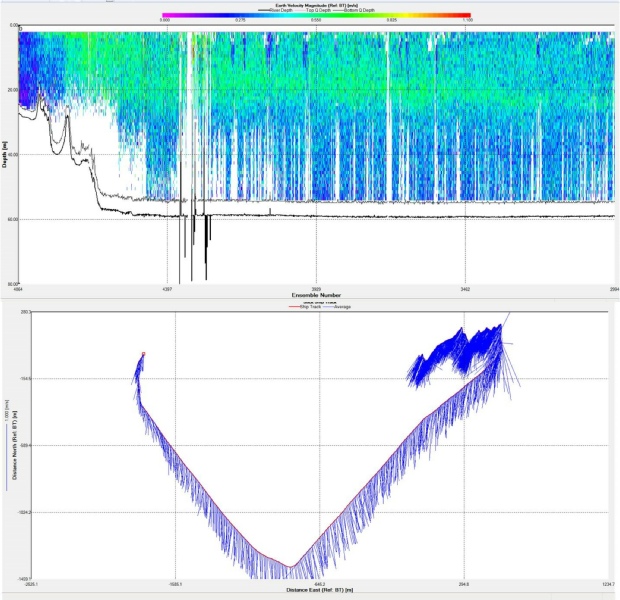
The coloured contour plot shows the earth velocity magnitude of the water column underlying the vessel. The ADCP line is undertaken in a transect, and so one graph displays distance on the x axis and depth along the y axis with the velocity plotted in colour, whilst the average flow direction graph shows distance east on the x axis, and distance north on the y axis with the ship track and average flow direction from the surface plotted on the graph.

Station 28: In the velocity plot for station 28, you can see that the majority of the water column is coloured blue, which means that the water is travelling at around 0.2 m/s. There are areas of lighter blue and also green that indicate velocities of 0.3-0.5 m/s. These areas of higher velocity occur just below the surface of the water, where the water is deepest. The plot for average flow direction shows that at the surface, the water is moving southwards very strongly, with only a few plot lines showing flow in another direction.

Station 28-29: In the velocity graph, you can see that between depths of 0 – 25m the velocity of the water column remains around 0.2-0.3 m/s in most places, and as the depth increases toward 40-60m, the velocity increases to 0.5-0.6 m/s in the centre of the water column. The plot for average flow direction shows that the flow is flowing very distinctly in a southwards direction, as the vessel moves southeast.

Station 29-30: The velocity graph shows that at the surface, the velocity varies between 0.275 – 0.825 m/s, and as the depth increases to 20m, the velocity reaches a maximum of around 0.7m/s across the whole transect, and over all water column depths.
Below 20m to the bed at around 60m depth the velocity decreases to 0.3m/s. Also, the velocity is highest at the surface where the water depth is at 40m. The average flow direction plot shows that the water is flowing towards the south very uniformly.

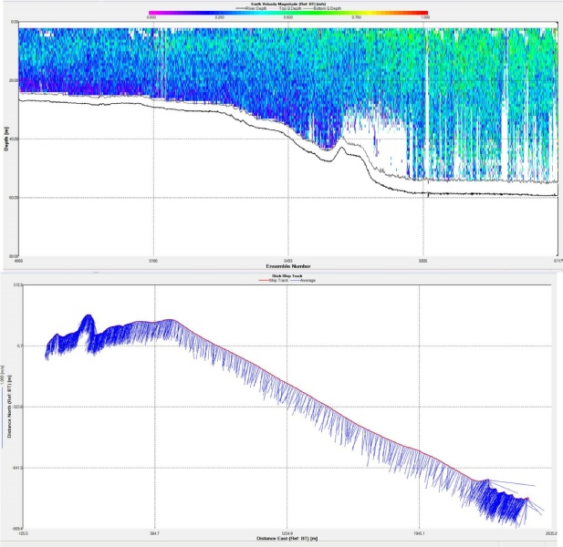
Station 30-31: The velocity graph shows that when the water depth is between 0-20m, the velocity remains at 0.25-0.3 m/s, and then when the water depth increases to around 60m the surface velocity increases to 0.5 – 0.65 m/s and the velocity at depth increases to 0.35 – 0.5 m/s. The lowest velocities are found just above the bed. The average flow direction plot show that the water is flowing southwards mainly, and at the beginning and the end of the transect the direction changes very slightly to south, south west.

Station 31-32: When the water depth is between 20-50m the velocity is mainly around 0.2 m/s, with some patches of near 0 m/s velocity, especially at the sea bed. As the water depth increases to around 50-60m depth, the velocity throughout the water column increases to around 0.3 m/s, with some patches of 0.4 m/s at the surface, and slightly slower velocities nearer the sea bed.On the average flow direction graph shows that the water is flowing in a southward direction consistently.

Station 32-33: On average the velocity plot shows that the water is moving at about 0.1-0.2 m/s throughout the water column, with higher surface velocities of 0.25 m/s where the water depth is greater than 40m. As the sea bed drops from 30-40m there is an increase to 0.2 m/s at the sea bed.
There are also two patches of surface water where velocities reach 0.5 m/s, where the water depth is less than 30m. The average flow direction plot shows that overall, the water is moving south. However, there is a lot of variability in the flow direction throughout the transect.

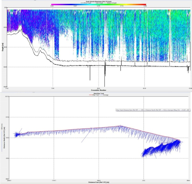
Station 33-34: The velocity plot shows that the velocities are on average around 0.15 m/s, with velocities reaching 0.3 m/s in patches where the water depth is below 25m. Where water depths are around 60m, velocities at the surface reach 0.5 m/s in small areas. The average flow direction plot shows that the water flows northwards, but there is a lot of variation, especially towards the end of the transect.

Station 34-35: The velocity graph shows that velocities are higher at the surface when the water depth is around 20m, and then when the water depth increases to around 60m, the surface has low velocities of around 1.75 m/s, whilst the velocity at depth varies between 0.4-0.6 m/s. The average flow direction graph shows that the water is flowing north – north west, however there is a lot of variation, especially at either end of the transect.

Station 35: The velocity graph shows that where the water depth is less than 20m, the velocity is higher at the surface than near the bed. Where the water depth increases towards 60m, then the surface velocity reduces and the velocity increases to 0.4 m/s near the sea bed. The average flow direction graph shows that the water is flowing north – north east, although there is a lot of variability in the data.

Chemistry

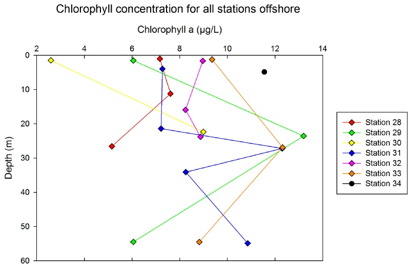
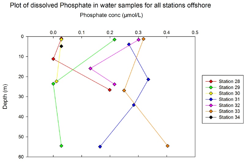
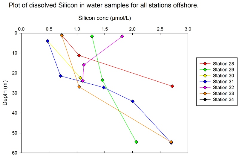
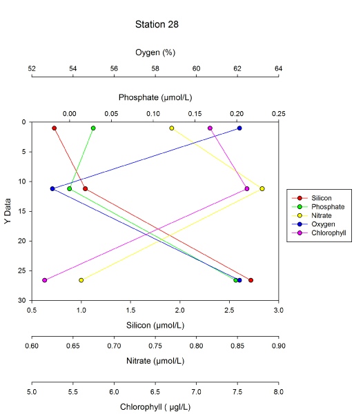
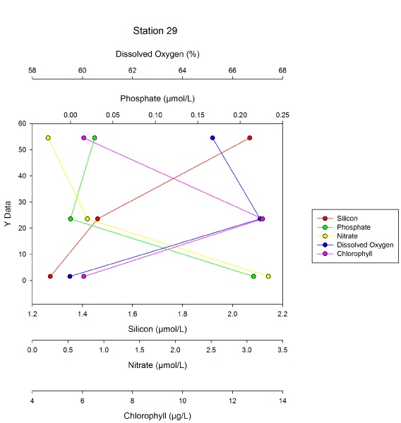
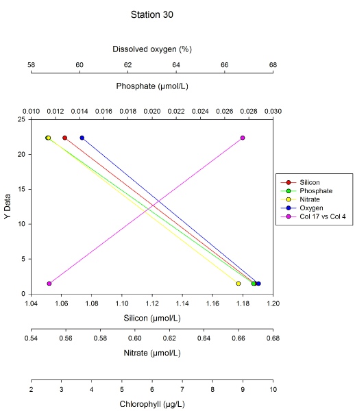
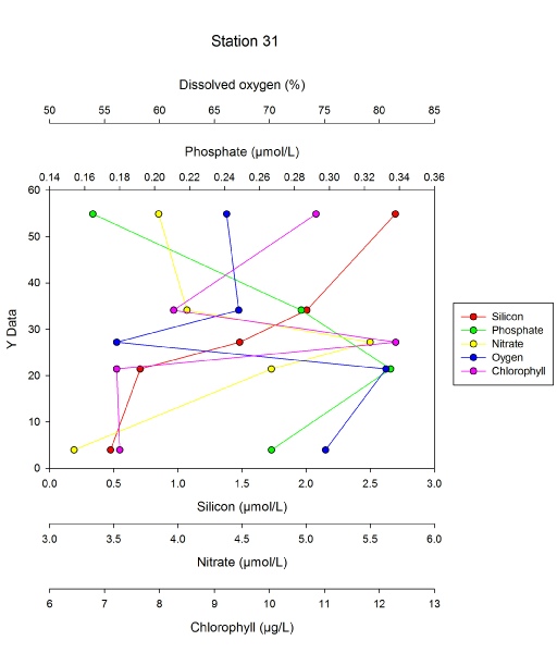
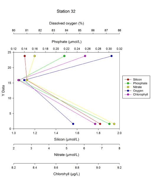
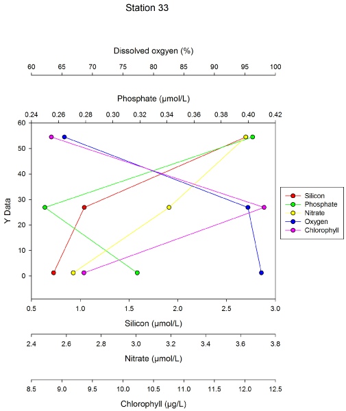
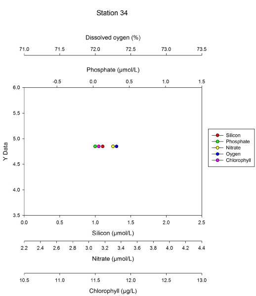
The first five figures within the chemistry section of graphs plot chlorophyll,dissolved oxygen, silicon,phosphate and nitrate against depth.

The deeper stations; 29, 31 and 33 all showed a deep chlorophyll maxima between 20-30m depth. These stations were all taken in the same location at 2 hour intervals throughout the day of 27/06/2014, this created a time series which ran through the low water time (11:47). Station 29 was taken during the ebb tide, station 31 around low water time and station 33 during the flood tide. The fact that station 31 was taken during low water may explain why there was an increase in chlorophyll at the deepest point, although it may also have been due to 5 depth samples being taken opposed to only 3 at the other stations. The deep chlorophyll maximum confirms the CTD readings of fluorescence which recorded a similar pattern. Stations 28, 30, 32 and 34 were all taken in a similar location in shallower waters, and had no distinguishable similarities. This may be due to shallow waters being more affected by tides than the deeper waters, also at some stations only 1 or 2 depth samples were taken meaning that it is difficult to get a high definition of the water column. In this case the CTD fluorescence reading may provide a more accurate representation of the water column. The highest chlorophyll reading (13.3µg/L) was in the mid water column at station 29 while the lowest (2.7µg/L) was at the surface of station 30.

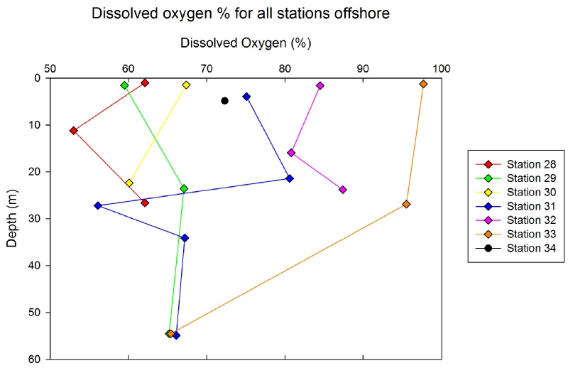
Phytoplankton are photosynthesising autotrophs, meaning they produce oxygen, therefore it can be expected that in regions of high phytoplankton abundance that dissolved oxygen will be the greatest. If true, the dissolved oxygen profiles should then follow the chlorophyll profiles closely. Station 29, 32 and 33 continue this theory as they had high oxygen in the mid water column. Station 28, 30 and 31 showed an oxygen minimum where there was a chlorophyll maximum which was unexpected. The highest dissolved oxygen (98%) was found at the surface of station 33 while the lowest value (52%) was at 10m depth at station 28.

At almost all stations the silicon concentration was lowest at the surface and increased with depth. This may be due to the presence of surface diatoms such as Leptocylindrus sp. which have siliceous frustules, the formation of which requires silicon. At greater depths there are less diatoms and therefor greater silicon concentrations. Station 32 is an exception to this rule as it had an abnormally high surface silicon concentration when compared with the other stations, meaning that the values at depth were lower than at the surface. The highest silicon concentration (2.7µmol/L) was found at the deepest point of station 28 whilst the lowest (0.45µmol/L) was found at the shallowest point of station 31.

There appears to be no pattern between stations as there is a large range in concentrations from station to station. The highest concentration (0.42µmol/L) was found at the deepest point at station 33, however at this depth in the other stations the concentrations found were low. The lowest concentration (0.0µmol/L) was found at the middle depths for station 28 at 11m and 29 at 23m.

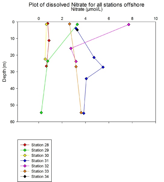
At stations 28, 30 and 33 the nitrate concentration appeared to be conservative throughout the depth profile, possibly representing a high degree of mixing. Station 29 and 32 appeared to have a higher concentration at the surface than at depth, this was unexpected as nitrate is normally a limiting nutrient and therefor normally depleted within surface waters where light intensity is high. Station 31 appeared to have a maximum nitrate concentration in the mid water column at 28m, therefor nitrate was not a limiting factor here, this may explain why chlorophyll concentrations were high at this depth. The highest nitrate concentration (7.8µmol/L) was at the surface of station 32 which appeared to be anomalous when compared with the other stations. The lowest nitrate concentration (0.1µmol/L) was at the deepest point of station 29.

Biology

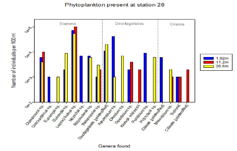
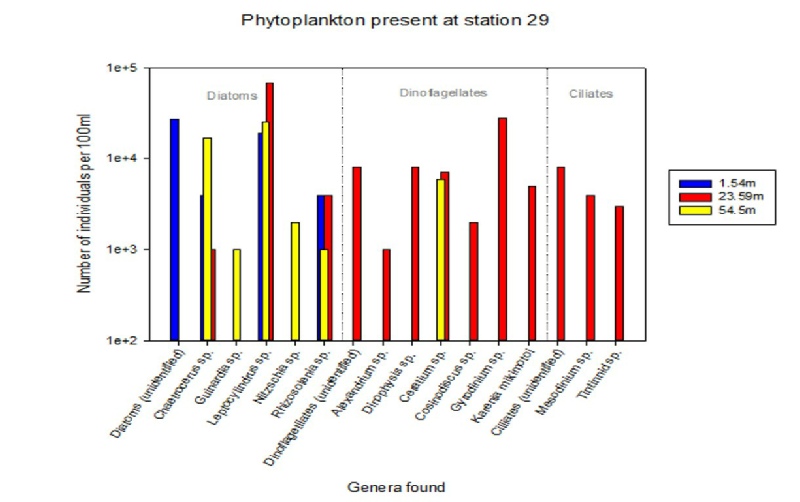
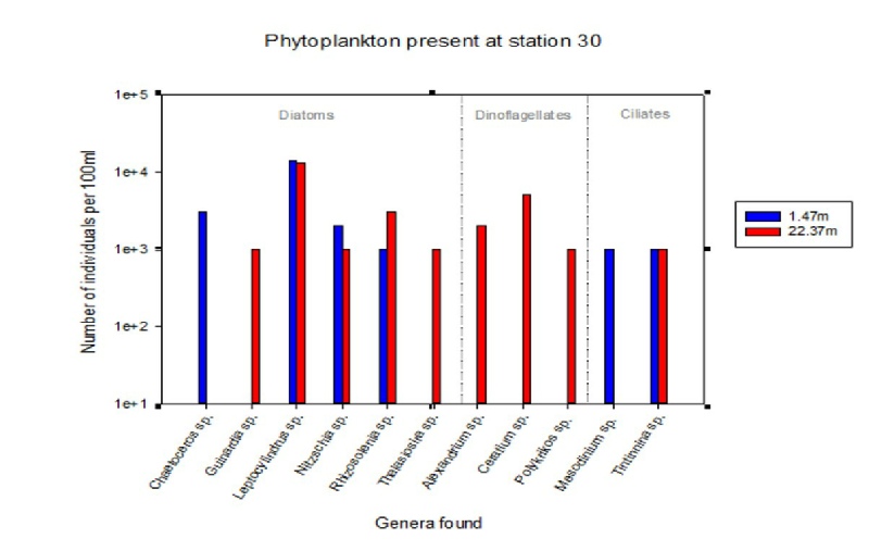
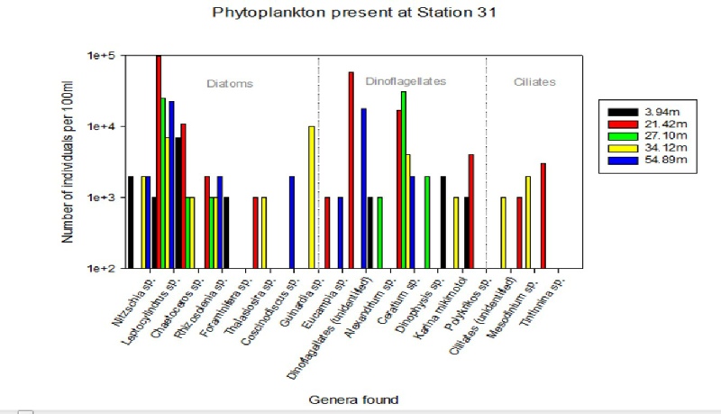
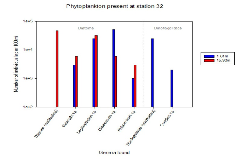
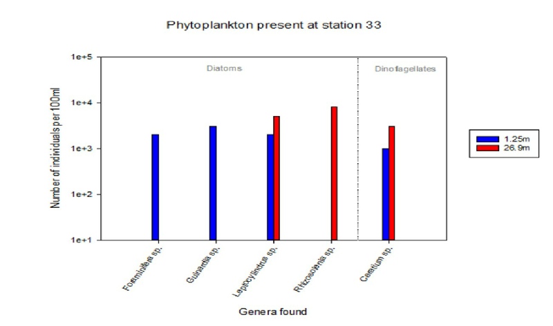
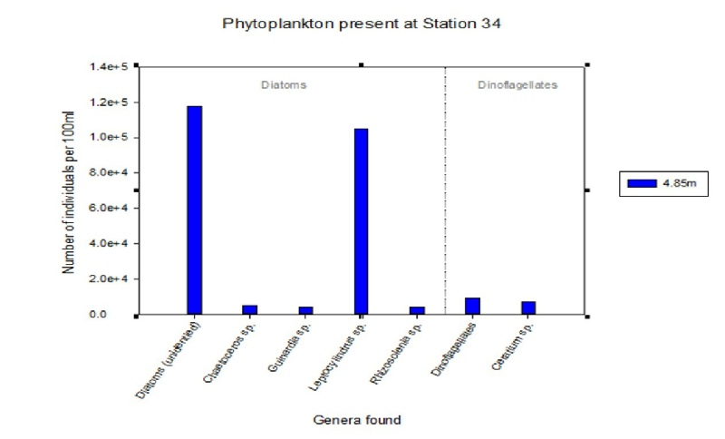
Phytoplankton: From the stations 28, 29, 30, 32, 33 and 34 it is evident to see that diatoms are the dominant type of phytoplankton in the water column. This is concordant with other research showing typical phytoplankton numbers at this time of year: late spring and early summer when the column is not completely stratified (Smyth et al. 2009). Though there is a strong presence of dinoflagellates (stations 28, 29, 31), particularly the species Alexandrium and Ceratium. This is indication that the water column is becoming more stratified as dinoflagellates thrive in stratified conditions (Cushing 1989) when the thermocline becomes more defined during the summer months (Knauss 2005).  Diatoms are also more prevalent in the surface waters (Stations 28, 29, 31, 33 and 34) particularly the species Leptoclyindrus, which is also the most abundant phytoplankton species with cell counts of near 10,000 per 100ml. Few other species reached or exceeded this number.  Though some stations showed the presence of ciliates they are visibly of lowest abundance compared to dinoflagellates and diatoms.

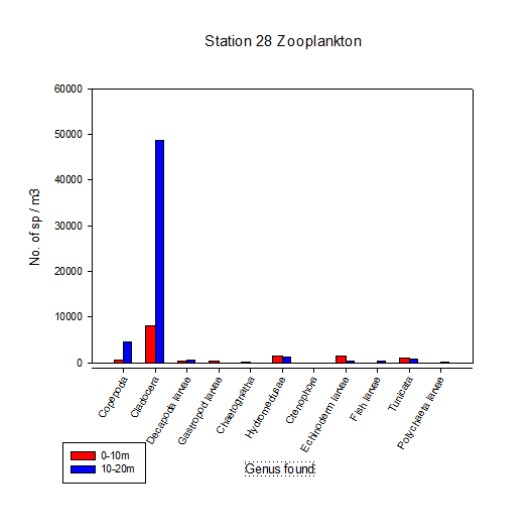
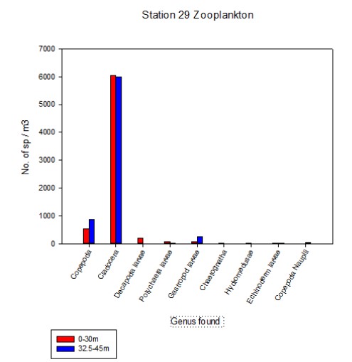
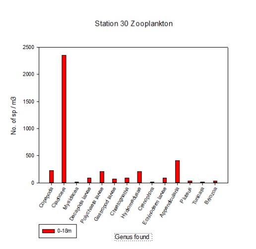
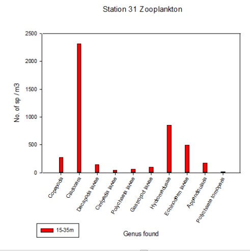
Zooplankton: Cladocera was the dominant taxa observed at all stations sampled, particularly at station 28 (49000 individuals m-3 between 10-20m. There were also more Cladocera at 0-10m than any other phyla, proving how prominent it was. The only other notable group at station 28 was copepoda.

There were significantly lower numbers of zooplankton at stations 29-33. However, Cladocera was still far more abundant than anything else. Hydromedusae were relatively abundant at station 31 (~800 individuals m-3) along with echinoderm larvae (500 individuals m-3).  Hydromedusae became more prominent during the later stations, suggesting their distribution is determined by tidal processes. There were no larvae found at more than 1000 individuals m-3 at any of the stations, implying they had a negligible impact on the biology.

References

Figure 1: Available at: http://www.visitmyharbour.com/harbours/channel-west/falmouth-marinas/charts.asp?cattype=5

               Accessed( 29/06/2014)

Cushing, D. H., (1989). “A difference in structure between ecosystems in strongly stratified waters and in those that are only weakly stratified.” Journal of Phytoplankton Research. Vol. 11 (1), pp. 1-13, doi: 10.1093/plankt/11.1.1

Knauss, J. A., (2005). “Introduction to Physical Oceanography.” 2nd ed. s.l.:Waveland Press.

Symth et al. (2009). “A broad spatio-temporal view of the Western English Channel observatory.” Journal of Phytoplankton Research. Vol 32 (5) pp. 585-601, doi: 10.1093/plankt/fbp128