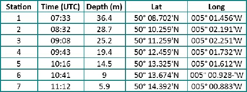
Meta data

Date: 27/06/2014

Time: 07:15-13.30

Location: Fal Estuary

Weather: 7/8 cloud cover

High tide: 06:56      4.7m

Low Tide: 19:08      4.9m

Overview

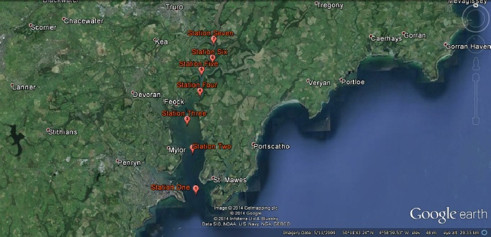
The aim of the investigation was to gain an understanding of the physical, chemical and biological conditions of the Fal estuary. This was achieved by creating a series of depth profiles at seven stations, starting at the mouth of the estuary, moving towards the riverine end.

Eulerian sampling allows identification of changes in various parameters in space along the estuary. The direction of the transect was chosen to ensure sampling was done against the ebbing tide to prevent sampling the same water as it flows in the same direction of the boat.

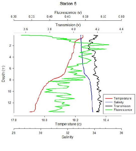
PLEASE NOTE: Due to a technical error, the original data for station 5 was not recorded from the CTD. On the return trip back to the mouth of the estuary a second CTD profile was taken in the same place as the first. However this data is out of time with the others and also in the flooding tide rather than the ebbing tide. Hence it cannot be directly compared to stations 1-7.

The Fal estuary is heavily contaminated with metals such as Cu, Cd, Zn and As (Brown et al., 2012) due to a long history of mining in the surrounding catchment area (Bryan and Langston 1992). The physical properties of the estuary affect the distribution and behaviour (chemistry) of constituents e.g. metals, which then impacts the biology of the area.

Methods

A CTD rosette was deployed at each station, recording fluorescence, temperature, salinity and transmission. Niskin bottles were fixed on the rosette in order to take water column samples for analysis of nutrients (nitrate, silicate and phosphate), phytoplankton, chlorophyll concentration and oxygen saturation. Surface and bottom samples were taken at each station and at stations 1-4 a further sample was taken when a CTD recording differed significantly at a particular depth.

A horizontal plankton net was deployed to collect zooplankton for counting and identification at stations 1, 4 and 7. Net trawls lasted five minutes, the mesh size of the net was 100µm and the open diameter was 50cm. An ADCP transect was conducted from bank to bank to provide a flow regime at each station. A Secchi disc depth recording was also taken at each station.

Sampling of station 5 was repeated after station 7 because of a malfunction with the CTD computer data. For this reason station 5 data cannot be used in the time series even if the results were similar it would not be a true time series.

*Phytoplankton and oxygen analysis samples were limited by a lack of equipment.

Laboratory Analysis

Please refer to Offshore (Link to offshore)  for the methods used to analyse the samples.

Figure 1: Map showing stations at which samples were taken in the Fal Estuary.

Results

Physical Properties

Temp

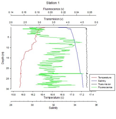
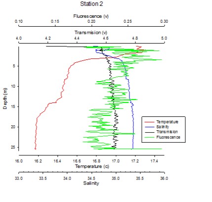
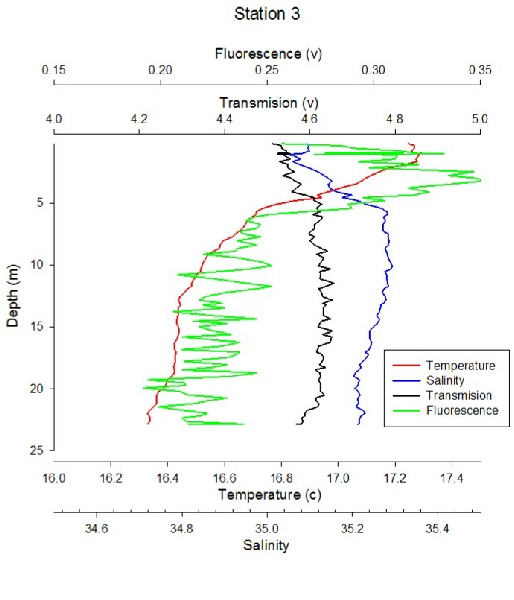
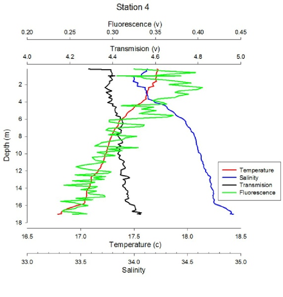
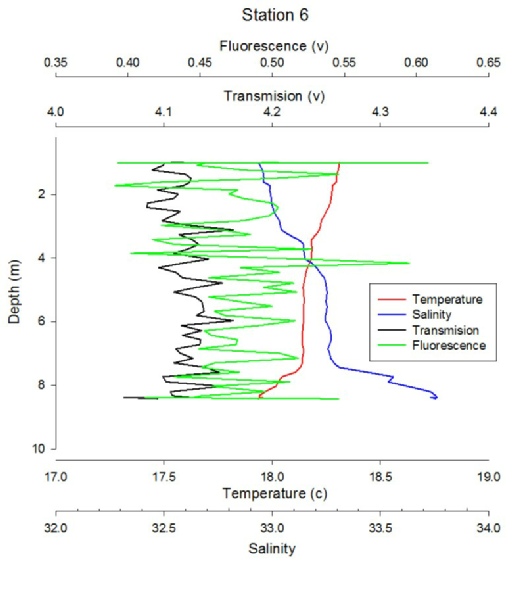
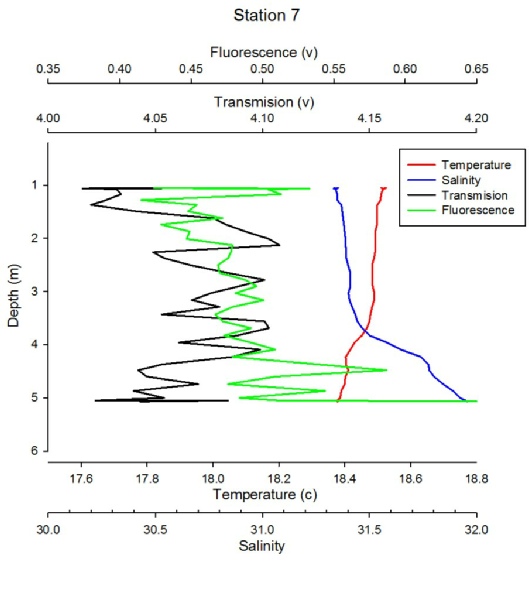
Temperature increased up the estuary with no exceptions. The maximum temperature at station 1 was in the surface waters (16.5oC) and was 2oC cooler than station 7 (18.5oC at 1m). Stations 6 and 7 were at least 0.6oC warmer than any other station in the transect. There is a general decrease in temperature with depth, however, stations 2 and 6 are the only stations with strong thermoclines. Stations 3 and 4 show a degree of stratification despite the lack of a thermocline. Station 1 appears to be the most well mixed in terms of temperature.

Salinity

Salinity is lowest in the upper estuary as expected, although it was particularly high (~31.5) considering low water was around the time of sampling. Station 1 is unusually low (33.4-34.7) as it was sampled within 90 minutes of high water. There is a mini halocline at station 1 at 1m but this doesn’t appear to correlate with any other physical characteristics at the station. Stratification becomes more apparent in the upper estuary. The highest salinity recordings were at the lowest depth recordings as expected.

Transmission

Transmission decreases up the estuary from 4.7v to 4.0v. The CTD recorded a lot of noise when measuring transmission, however, it is uniform with depth at all stations besides station 3 where it increases with depth. Transmission gives the inverse of turbidity, which implies greater turbidity at the mouth of the estuary.

Fluorescence

The CTD measures fluorescence, which is used as a proxy for measuring chlorophyll a; higher fluorescence implies a higher chlorophyll levels. Fluorescence increases at a relatively constant rate towards the riverine end of the estuary. A fluorescence maxima occurs in the upper 5m of the water column at most stations followed by a slight decrease with depth. Station 1 does not correlate with the rest of the data as it was lowest in the upper 4m and its maxima was at 7.5m. Station 1 and 2 also exhibit deep chlorophyll maxima at 22.5m and 25.3m respectively. There is also a maxima at 3.5m, just above the thermocline, at station 2, which is expected.

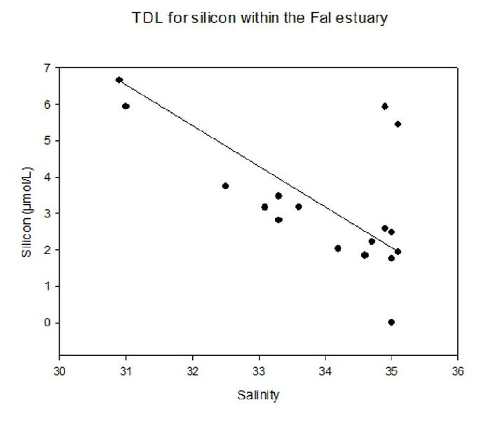
Chemistry

Silicon: Lowest concentrations of silicon in the mid estuary (0-3 µmol/L) . The estuarine mixing diagram reinforces this and suggests that silicon is behaving non-conservatively as it does not plot down the Theoretical Dilution Line. As the plots are below the TDL there is removal of silicon between the mid-estuary and the mouth. There are two unusual results at the mouth of the estuary where silicon concentration is abnormally high; at station 1 at the surface and on the bottom (5.4 and 4.9 µmol/L respectively). There does not appear to be a regular pattern of silicon concentration along the estuary.

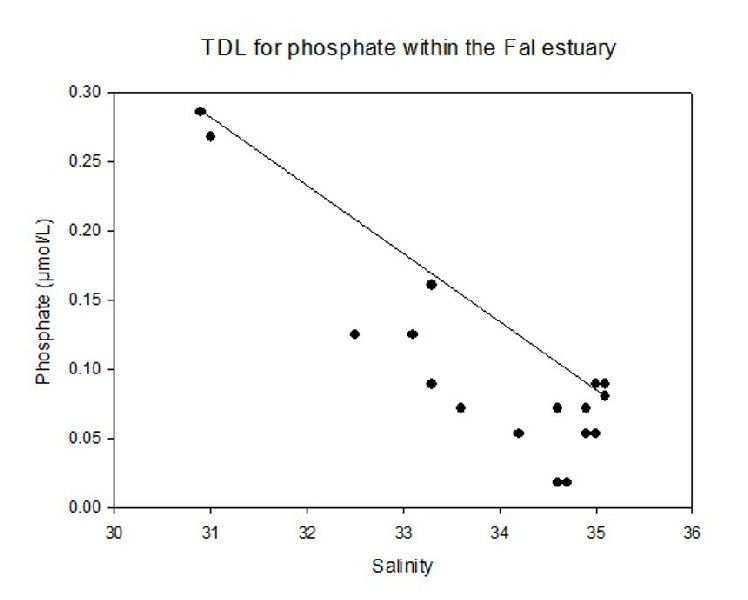
Phosphate

Phosphate also shows removal in the estuary, implying it is involved in biological or chemical reactions. Concentration was as low as 0.00-0.07 µmol/L at the middle stations. At station 7 phosphate was much more concentrated than the other stations (~0.27 µmol/L).

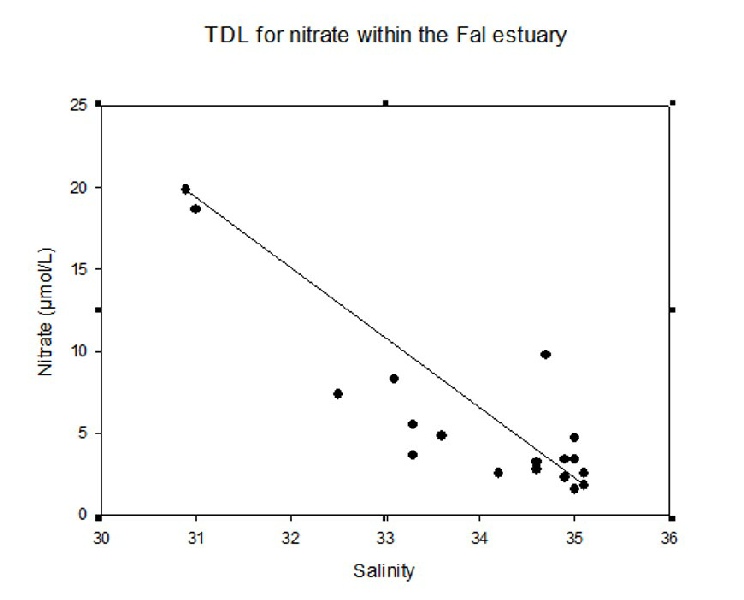
Nitrate

Nitrate was behaving non-conservatively at mid-salinities, along with the other nutrients. However, it started to behave conservatively towards the mouth of the estuary as the points are clustered around the TDL. Station 7 had a considerably higher nitrate concentration (~19 µmol/L) than any of the other stations.

Dissolved O2

Dissolved O2 concentration increased towards the riverine end of the estuary. Concentration decreased with depth at stations 1—4 but increased at the bottom reading at stations 6 and 7. Station 5 appears abnormally high relative to stations 6 and 7.

Chlorophyll

The results for chlorophyll are fairly analogous with dissolved Oxygen, suggesting their concentrations are controlled by phytoplankton populations. Chlorophyll concentration increases at each station from station 1 (~0.1-0.4 µg/L) to station 7 (~9 µg/L). There was less chlorophyll in the surface waters but the remaining water column is fairly uniform.

Local Behaviour of Constituents

Station 1: High concentrations at the surface and bottom with minima at the intermediate readings. Phosphate is the only constituent that followed the opposite pattern.

Station 2: All constituents decreased in concentration with depth except for phosphate, which followed the opposite pattern again.

Station 3: There was nutrient depletion in the surface waters. Concentrations increased with depth except for silicon, which decreased rapidly between the intermediate and bottom readings. Oxygen saturation and chlorophyll concentration decreased with depth.

Station 4: Levels of all constituents were high at the surface and all decreased with depth except for silicon, which had a uniform distribution throughout the water column.

Station 5: Nitrate, phosphate and chlorophyll decreased with depth, whereas silicon increases. There was only one reading for Oxygen concentration so it is not possible to analyse its vertical behaviour.

Station 6: Nitrate and Oxygen increased with depth and silicon and phosphate decreased with depth. The phosphate reading was very similar at the surface and on the bottom but cannot be described as uniform as there were only two readings.

Station 7: Oxygen and chlorophyll concentration both increased with depth while all the nutrients decreased towards the bottom.

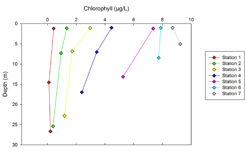
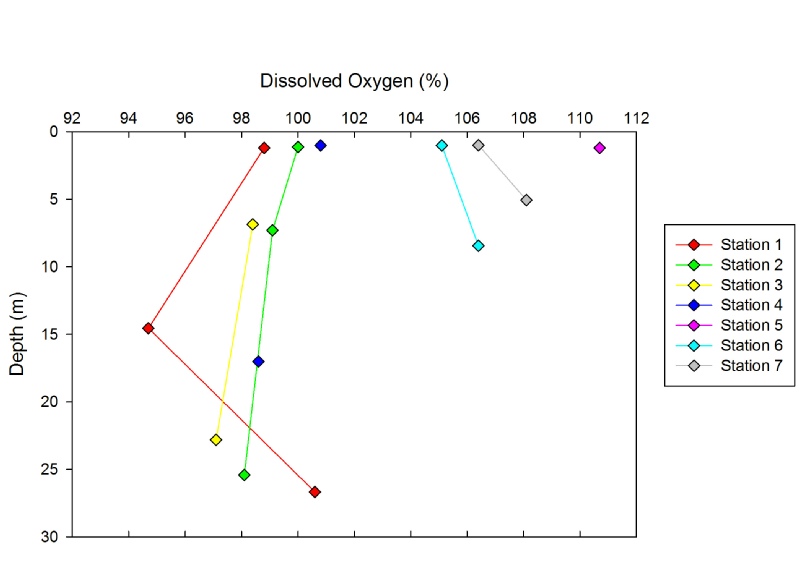
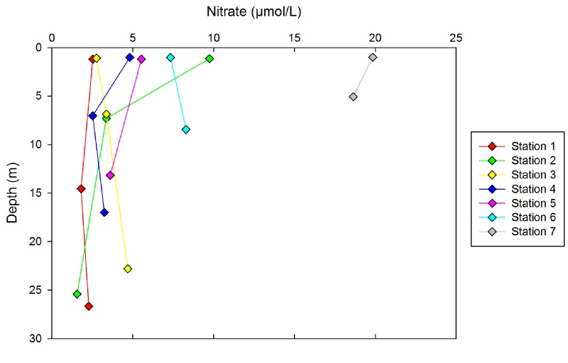
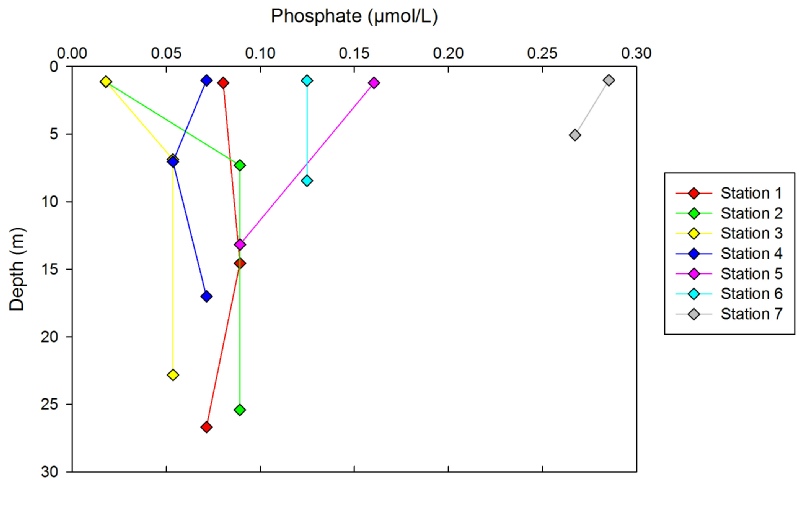
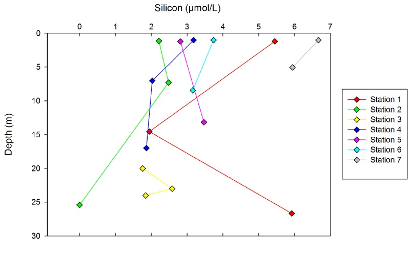
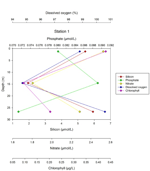
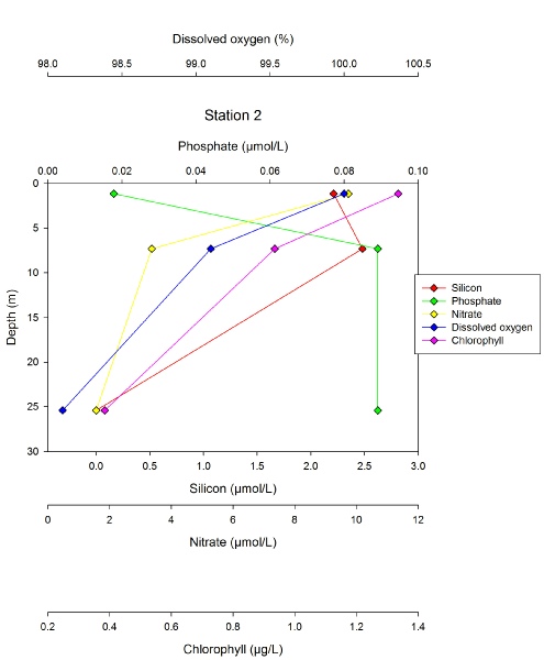
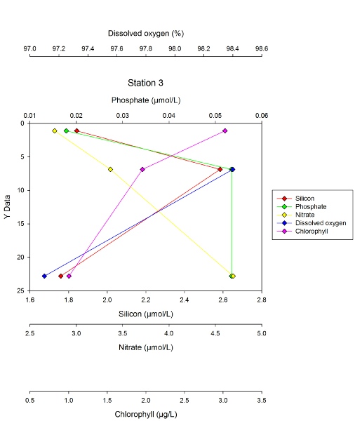
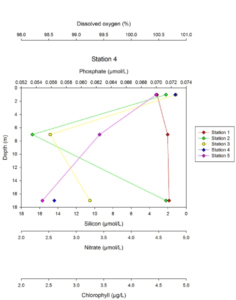
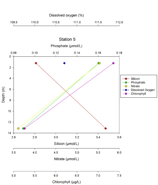
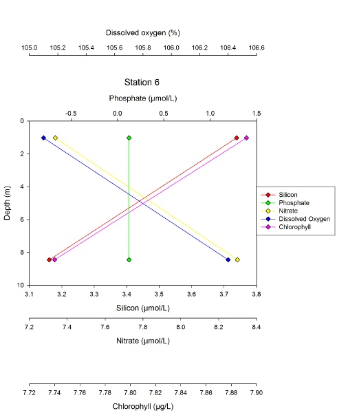
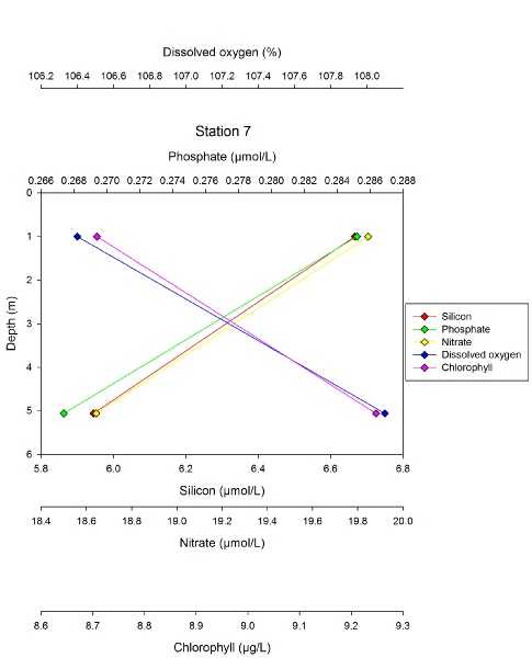
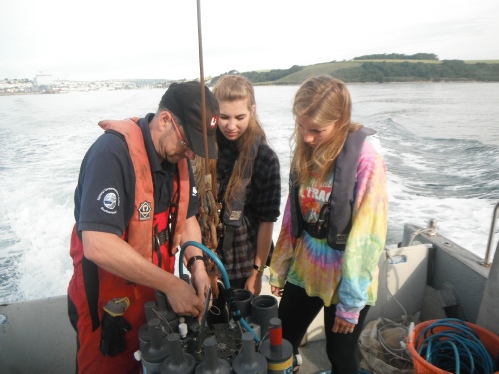
Figure 2: Preparing to deploy the CTD by resetting the Niskin bottles.

Richardson’s Number (Ri)  

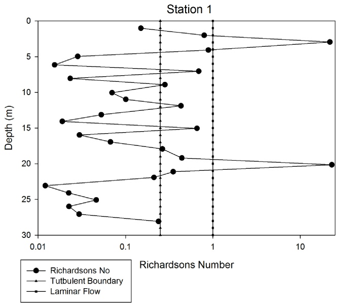
Richardson’s number is a non-dimensional ratio of the density gradient to the velocity shear (Knauss, 2005). The smaller the Richardson’s number the greater the tendency for vertical mixing meaning increased turbulent flow. If the Richardson’s number becomes less than 0.25, shear waves are generated along the interface so the two fluids become unstable and therefore break.

Station 1:Station 1 has turbulent flow because all Richardson’s numbers are below 0.25, most of the numbers stay between 0.00 and 0.05 fluctuating alternately, however at 15m depth and our final depth the Richardson’s numbers increase to nearly 0.15 indicating a decrease in turbulent flow.

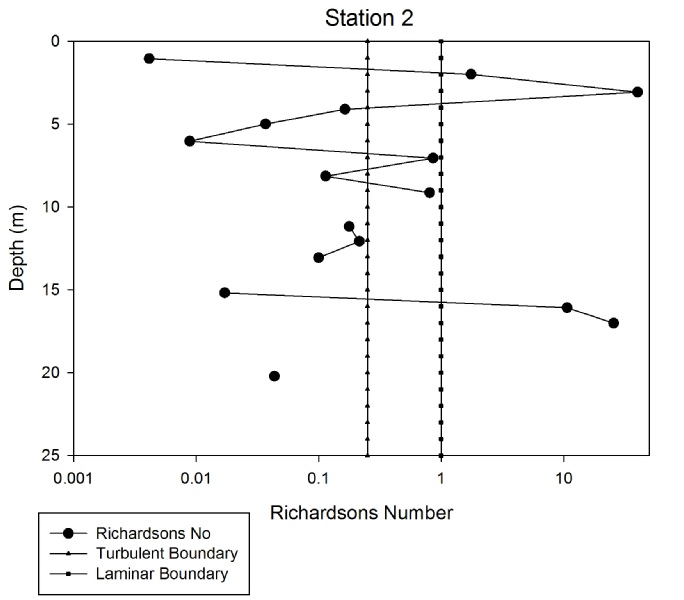
Station 2: At this station the Richardson number stays quite constant at roughly 0.00, there are a few fluctuations at 3m, 13m and 17m depth however none of these increases in Ri ever rise above 0.05, indicating the water column is turbulent and vertical mixing between the two water masses is occurring.  

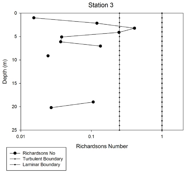
Station 3: The upper 5m of the water column has a fluctuating Richardson’s number but once again never rising above 0.05. Below 5m the Richardson’s number stays constant at roughly 0.00, indicating a turbulent flow again meaning shear waves are generated along the interface of the fresh water mass and salt water mass.

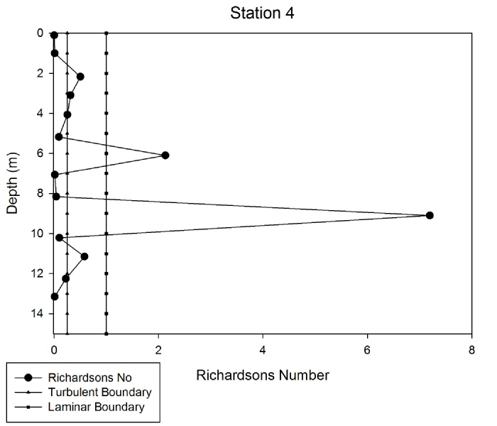
Station 4: Station 4 is concordant with the previous stations, with none of the Richardson’s numbers rising above 0.05 which indicates there is turbulent flow as all values are below 0.25 suggesting vertical mixing. There is an increase in Richardson’s number at 11m but only by 0.04 therefore there is no significant change in the vertical mixing of the water.

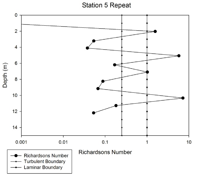
Station 5 Repeat: The Richardson’s number peaks at 7m depth but follows the trend of the previous stations by not increasing to over 0.05. This shows there is no change and shear waves are generated along the interface of the two water masses, so as we go up the estuary there is no change in the turbulence of the water.

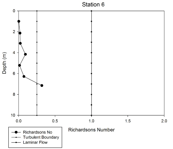
Station 6: Station 6 has fewer points than previous stations, this is due to the decrease in water depth however there is still a similar trend with Richardson’s number, with depths up to 6m staying at the 0.00 mark indicating turbulent waters. At 7m there is an increase in the Richardson’s number to nearly 0.10, however this number is still under 0.25 which is the cut off for vertical mixing and turbulent waters suggesting the water column is very well mixed however on the bottom of the sea floor there is a slight decrease in vertical mixing meaning turbulence decreases slightly.

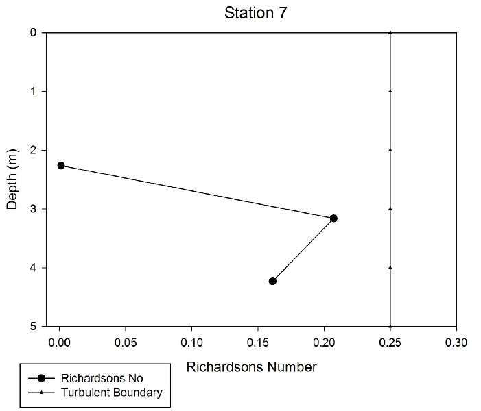
Station 7: The water column is still turbulent because all values are below 0.25 suggesting a vertically mixed water column. However at depths 3 and 4 the Richardson’s number decreases suggesting a slight decrease in turbulence meaning less vertical mixing in the water column therefore there is less of an interface between the two water masses.

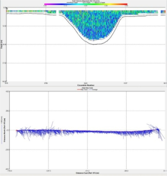
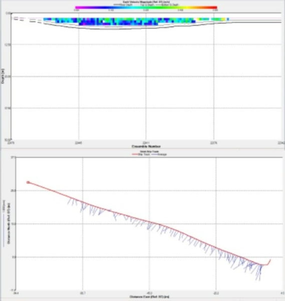
ACDP

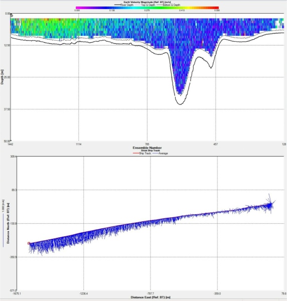
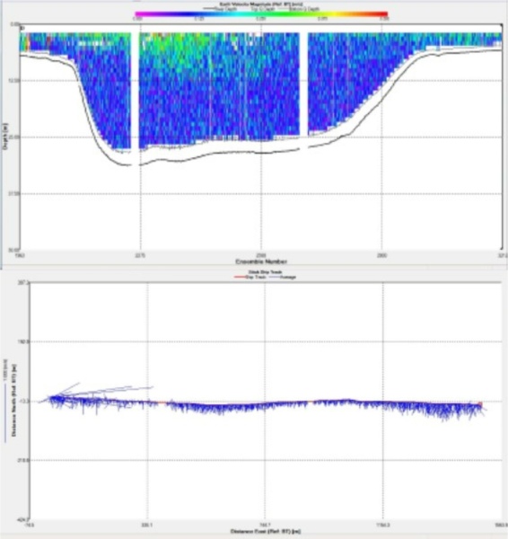
The coloured contour plot shows the earth velocity magnitude of the water column underlying the vessel. The ADCP lines were undertaken along transects, and plots distance against depth with the velocity plotted in colour. The average flow direction graph plots distance east against distance north with the ship track and average flow direction from the surface plotted on the graph. The tide was ebbing during sampling of the estuary, which explains the direction of water flow.

Station 1: The velocity graph shows that most of the water column had velocities of around 0.15 m/s, including a deep valley of 30m. There were velocities of 0.3-0.5 m/s found at the surface water, when the water depth was less than 12.5m. The average flow direction graph shows that the water was moving southwards consistently.

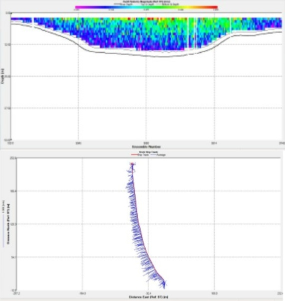
Station 2: The velocity plot shows that the velocity was consistently low throughout the water column, with a higher surface velocity directly above the deepest area of the water column. The average flow direction graph shows that the water was moving south fairly consistently, with a few variability’s in the data.

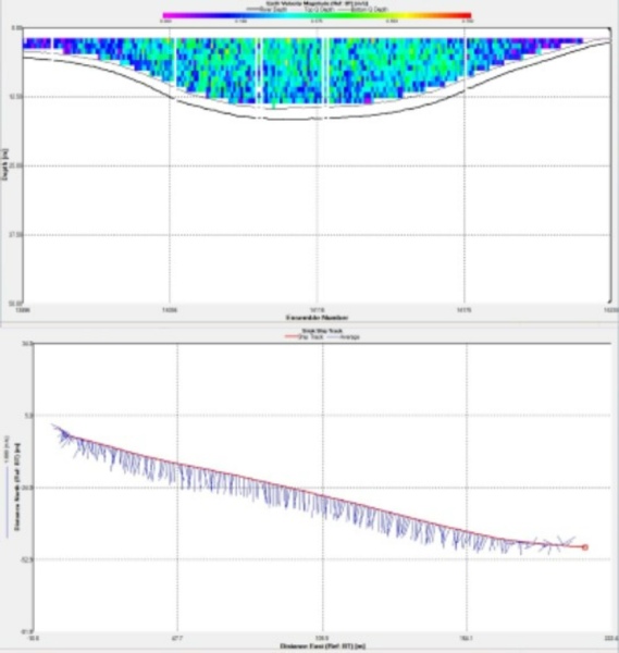
Station 3: The velocity graph shows that the water had the highest velocities at the surface, at around 0.2 m/s, and the lowest velocities were found where the water depth was around 20m, at the bed of the estuary. The average flow direction plot shows that the water was moving southwards, however the data is not fully consistent as some plot lines show the water to be moving northwards.

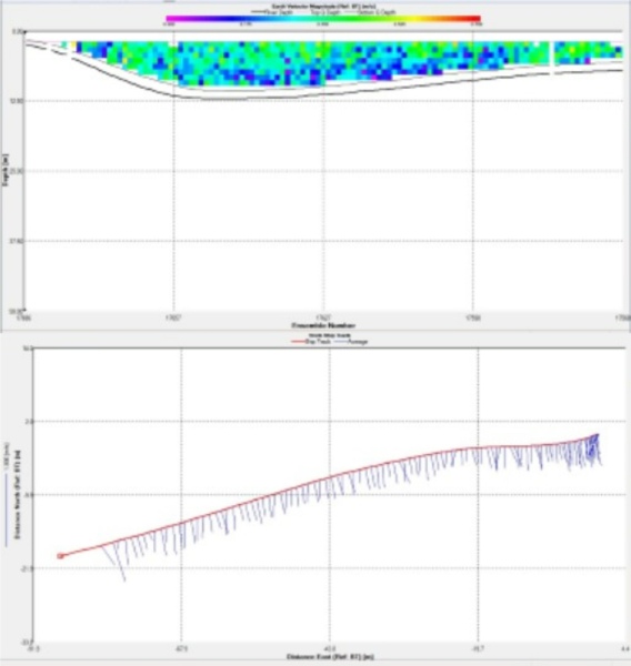
Station 4: The velocity graph shows that velocities were low near both the surface and the bed. In the deep water column, the surface waters show increased velocities of 0.4 m/s. The average flow direction graph shows that the water was moving southwest consistently.

Station 5: The velocity graph shows that the velocity was fairly consistent throughout the water column, ranging between 0.1 m/s and 0.25 m/s. The average flow direction graph shows that the water was moving southwards very consistently.

Station 6: The velocity graph shows that the water column was consistent in velocity between 0.15 m/s and 0.3 m/s all the way through the water column. The highest velocities were found at the surface.vThe average flow direction graph shows that the water was travelling southwards very consistently with almost no fluctuations.

Station 7: The velocity graph shows that the velocity was higher at the surface, with typical values of 0.25 m/s, with lower velocities at the bed of the estuary such as 0.15 m/s. The average flow direction plot shows that the water was travelling south west very consistently.

Biology

Zooplankton

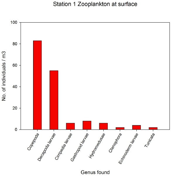
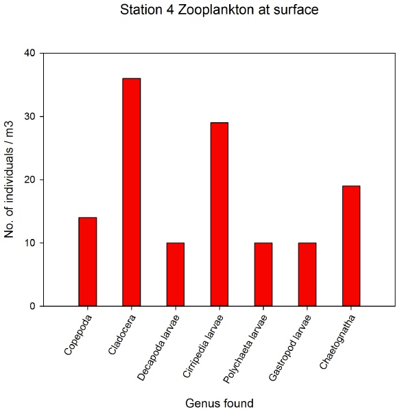
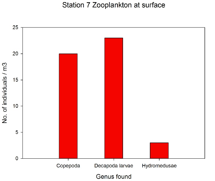
Copepod larvae were dominant at station 1 (82 individuals m-3) along with decapod crustacean larvae (53 individuals m-3). There are several other species from different phyla present, however, they are not abundant and therefore not as likely to contribute to the biology of the water column. Copepods are still present at station 4 but are much less abundant . Cladocera are the most abundant (36 individuals m-3), followed by Cirripedia larvae (28 individuals m-3). There is much more of an even spread between zooplankton taxa in general as seven different groups were observed at 10 individuals per m3 or greater. Zooplankton diversity is significantly less at station 7 in terms of abundance and number of taxa, as expected. Despite this, copepods and decapod larvae are present at 20 and 23 individuals per m3 respectively.

These results suggest that copepods are able to survive at either end of the estuary despite the differing conditions. Samples would have needed to have been taken at the other stations to be able to make firmer assumptions about the zooplankton populations of the Fal estuary.

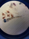
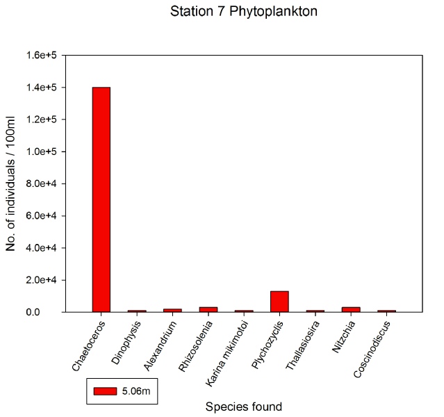
Phytoplankton

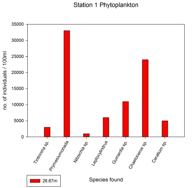
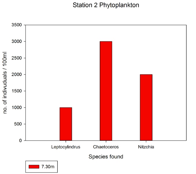
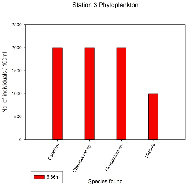
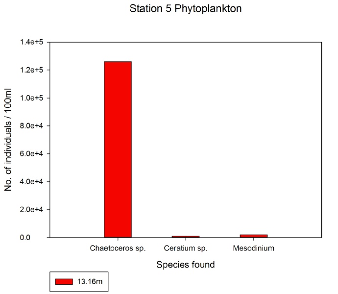
Phytoplankton samples were taken at varying depths at different stations depending on the physical structure of the water column, therefore, it is difficult to compare between stations.

Prymesiumonada was highly abundant at station 1 at 33000 per 100ml, however, it was not present at all at any of the other stations. This could be down to the depth of the sample being far deeper than at any other station. Chaetoceros sp. was also very common at station 1 at 24000 cells 100ml-1. Phytoplankton abundance in general was much lower at stations 2 and 3 despite the fluorescence readings being higher than station 1. Chaetoceros was also vastly abundant at stations 5 and 7 (126000 and 140000 cells 100ml-1). Plychozyclis was abundant at station 7 relative to everything but Chaetoceros (13000 cells 100ml-1).

References

Knauss, J. A., 2005. Introduction to Physical Oceanography. 2nd ed. s.l.:Waveland Press.

Brown, M. T., Newman, J. E., & Han, T. (2012). Inter-population comparisons of copper resistance and accumulation in the red seaweed, Gracilariopsis longissima. Ecotoxicology, 21(2), 591-600.

Bryan GW, Langston WJ (1992) Bioavailability, accumulation and effects of heavy metals in sediments with special reference to United Kingdom estuaries: a review. Environ Pollut 76:89–131