Home Estuary Pontoon Offshore Habitat Mapping

Meta Data

Date: 01/07/2014
Time: 7.30

Location: Start: 50°08’662”N, 005°01’435”W

             Finish: 50°14’392”N, 005°00’882”W

Low Tide: 11.17 (1m), 23.43 (0.9m)

High Tide: 04.35 (4.6m), 16.57 (4.7m)

Wind: 90° 6.2ms-1

8 octants cloud cover reducing to 5 octants

(All times in UTC)

Abstract

Sampling up the Fal estuary a survey was conducted which took secchi disc measurements, CTD water samples and ADCP horizontal transects. Samples were taken across 7 different stations, from offshore to the river end. Temperature, salinity, fluorescence, transmission, velocity magnitude, backscatter, nutrients, phytoplankton and zooplankton were taken at each station. From the data collected, flushing time, residence time, Richardson number and light attenuation coefficients were calculated. Charts, graphs and mixing diagrams were compiled using the data and calculated values. From the results, it was found that the estuary seemed to have a well-mixed structure offshore and became more stratified towards the river end, however the Ri number graphs seem to slightly contradict the depth profiles taken with the CTD as the Ri number suggest that, at certain stations, parts of the water column are stratified, when the depth profiles suggest they were well-mixed. There were no definite conclusions made concerning the behaviour of nutrients in the estuary, this was difficult because the data only consisted of salinities 29-35. Although, using incomplete mixing diagrams, predictions were able to be made for the behaviour of each nutrient, silicon showing conservative tendencies similar to nitrate whereas phosphate was non-conservative. However as eluded to these diagrams were not conclusive. Patterns were also found between light attenuation and turbidity, as turbidity increased up the estuary, light attenuation decreased.

Introduction

The Fal estuary is a classic ria formed after the last ice age – when rising sea levels flooded the river valley. It stretches approximately 18km from Pendennis Point at the English Channel to its tidal limit at Tresillian on the River Fal. The majority of the estuary is contained within a large tidal basin on the outer estuary called Carrick Roads. A deep channel (reaching a maximum depth of 34m) runs through this basin getting progressively shallower as it goes inland.

The estuary acts as a transition zone between the freshwater input from the River Fal and its tributaries and the salt water from the English Channel. The combination of these two waters creates a complex system, its’ properties dependent on a wide range of factors including tidal range, freshwater input, geography (such as depth and area), weather (especially precipitation and wind) and chemical (nutrients and pollutants) input from the land.  (Simpson, 1990)

The aim of this survey is to establish how the concentrations of various nutrients change, moving through the estuary. This will enable us to examine several physical properties of the estuary such as how well mixed it is, the influence of the tide and what the flushing time is. Samples of phytoplankton and zooplankton will also allow us to compare the communities found within the estuary to those sampled during the offshore survey.

Methods

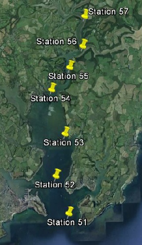
Starting from the mouth of the estuary near Black Rock, seven stations were selected to characterise the different sections of the estuary as well as possible. It wasn’t possible to go any further inland than station 7 as the depth beyond this point was too shallow for the Bill Conway to operate safely. The instruments used to collect the data were:

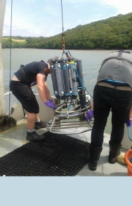
Rosette Sampler

A rosette sampler equipped with 6 Niskin bottles and a CTD was deployed at each station giving readings at 3 depths (except at station 7 where only 2 were taken due to shallow water). As with the measurements taken offshore the CTD profile created on the descent of the rosette was used to determine where to take samples on the ascent.

Plankton Net

A plankton net (mesh size 200µm, diameter 0.5m) was deployed at the surface for 3 of the 7 stations (1, 4 and 7).

Secchi Disc

The turbidity of the water was analysed using a Secchi disc, allowing us to calculate the photic zone (3 x the depth where the Secchi disc is no longer visible).

Laboratory – Conway

The samples taken from the Niskin bottles and the plankton nets were all processed on board the Conway, ready to be analysed in the on shore laboratory. Phytoplankton, phosphate, nitrate, silicon and chlorophyll samples were taken from each depth but due to a lack of bottles, oxygen samples were only taken from the surface and the bottom.

Laboratory – Falmouth

As with the offshore study the preserved samples were analysed to give O2, phosphate, nitrate, silicon and chlorophyll concentrations. Stereo and light microscopes were used to calculate the concentration of zooplankton and phytoplankton.

Flushing and residence times

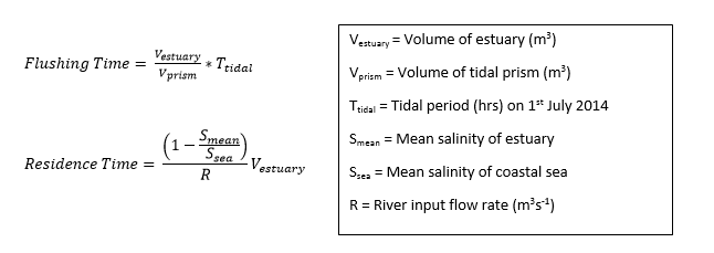
An estimation of the flush and residence times were calculated using a combination of archive and survey data from the estuary survey using the following equations:

To estimate the area of the estuary, a rough outline was traced using Google Earth Pro which then calculated the enclosed area (see Image 3). The average depth of the estuary was estimated by taking an average of the depth recorded at all 7 stations and multiplying with the area.

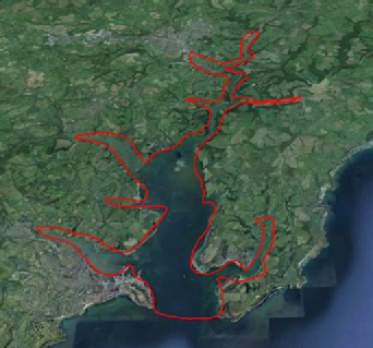
Image 3| An outline of the Fal Estuary made using Google Earth Pro,

used to calculate the estuary area (approximately 24.6 km2)

The volume of the prism was calculated by multiplying the area of the estuary with the tidal range (the difference between high and low tide on 1st July 2014), and the tidal period is the time between the two high tides on the same date.

The mean salinity of the estuary is an average of the salinity recorded at each of the 7 stations and the mean salinity of the sea is an average of all salinities recorded during the offshore practical. River flow data was obtained from the Centre for Ecology & Hydrology and is the average daily flow rate between 1978 and 2009 of the Rivers Fal and Kenwyn.

Results

Figures 1-14

Figures 1-7 show the depth profiles of fluorescence, temperature, salinity and transmission for stations 51-57 up the Fal estuary; with station 51 contained the information for seawater end member while the river end member data was provided by external source.  Maximum depth of water column decreased gradually from 34.95 to 3.21m (stations 51-57; Figures 1-7).

Fluorescence

The fluorescence data in Figure 10 presents and indicates a trend of increasing chlorophyll detected in overall water column from lower to upper estuary, however such levels fluctuated across depths at all stations. While Figure 1 shows the chlorophyll levels fluctuated around the stable mean throughout the water column at stations 51-53; Figure 4 and 5 present a slight variation in the fluctuated chlorophyll level across the water column at station 54 and 55.

Figure 4 shows a slight trend of decrease in such fluctuation throughout water column at station 54. Figure 5 shows a slight increase in the fluorescence (chlorophyll) level from 1.02 to 2.85m depth (0.426 to 0.543mg/L3), the level then remained relatively stable from 2.85m to the bottom of water column (11.94m).

Figure 6 shows similar trend as shown in Figure 5 at station 56 with a larger increase in chlorophyll level measured at the surface; from 0.84 to 2.31m the fluorescence (chlorophyll) level increased from 0.332 to 0.583mg/L3. The fluctuated chlorophyll level was relatively constant across depths at station 57.

Temperature

Similar to the fluorescence data, there was a trend of increase in the overall temperature in water column from lower to upper estuary as presented in Figure 8. Figures 1-4 show stations 51-54 shared similar bottom temperature values (varying between 16.553 and 16.645oC). However the vertical temperature profiles progressively deviated from almost no temperature difference (0.002oC) between surface and bottom at station 51, to 0.720oC difference at station 54 (with higher temperature values detected on surface at each station from stations 51-54)

Figures 5-7 present a gradual increase in the bottom temperature values measured from 17.825 to 18.713oC across stations 55-57. While Figure 5 shows a very slight inverse exponential decrease in temperature across depths at station 55; Figure 6 and 7 show a decrease in temperature only at the middle depth, with the temperature values in upper and lower water column remained relatively stable at both station 56 and 57.

Salinity

Salinity profiles at all stations (Figure 9) show a similar transition in parameter along the Fal Estuary as shown in the temperature profiles across stations (Figure 8), despite the fact that the overall salinity in water column decreased upstream. Similar bottom salinity values were detected at stations 51-54 (varying between 34.908 and 34.991). Figure 1 shows a gradual increase in salinity from 34.331 to 34.928 at station 51. Figure 4 displays an increase in salinity at the middle depth at station 54 (from 34.431 to 34.728; 6.09 to 8.15m), while the salinity in the upper and lower water column remained relatively stable at station 54. Figure 2 and 3 show the salinity level remained constant throughout the water column at stations 52 and 53. Similarly, Figure 5 also displays constant salinity level across depths at station 55, but with overall lower salinity level detected compared to stations 52-54 (Figure 9).

Figure 9 shows a rapid decrease in the overall salinity in water columns as stations moved upstream from station 55. Similar to station 54, the salinity increased at middle depth at station 56 and 57. However, a slight increase in salinity across the bottom water column of station 57 was noticed (Figure 7), otherwise remained stable across sectioned water column. Station 57 had greater increase in salinity (1.082, from 2.18 to 2.49m) compared to station 56 (0.23, from 5.11 to 7.33m).

Transmission

Transmission data presented in Figure 11 represents the variation in the turbidity level along the Fal Estuary, i.e. as transmission increases the turbidity level decreases. Similar to the fluorescence data, the measured transmission values fluctuated throughout the water column at each station. The overall turbidity level across water column increased slightly from stations 51-53, then a greater increase in such level was observed from stations 53-57 (see Figure 11).

The transmission levels were constant across depths at stations 51-56 (see Figures 1-6). At station 57, the level was constant from surface to 2.1m, then increased slightly by 0.161V to 3.21m.

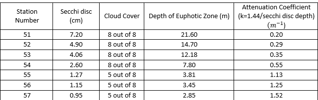
The secchi disc depth and attenuation coefficient have negative correlation because, as depth decreases moving up the estuary (station 51-57) from 7.2m to 0.95m, the attenuation coefficient of light increases from 0.2to 1.52. There is greater increase in light attenuated between stations 54 and 55 than any other station. Moreover, cloud cover decreased from 8/8 to 5/8 after Station 54 and then remained the same. The depth of the euphotic zone becomes less deep at the river end compared to offshore.

Figures 15-28

ADCP Data

Figure 15 shows a horizontal transect across the estuary at the seawater end member (station 51). As shown by the outline and depth figures, in the outer sides of the estuary it was relatively shallow at around 9m, whereas in the central channel it goes to depths of 30m and more. The backscatter values were very low; 60-70 dB throughout the transect at varying depths of around 6m, highest values were recorded nearer the surface of up to 96dB in 3 different places along the transect. At the seabed at ensemble number 5443 there was also an area of high dB of up to 75.

A similar transect can be seen at station 52 (Figure 16) and, similarly to Figure 15, has a deeper central channel. The deepest part of the central channel contains minimum backscatter values, at 64 dB at 26.3m. Again similar to the transect at station 51, Figure 16 shows maximum values of backscatter near the surface, however these maxima were not along the whole transect but were above deep channel. These values were up to 98dB in places.

The transect- as shown by Figure 17- was taken at station 53 and shows the deep channel was far off to one side, containing middling values, around 74dB. The relatively shallow side, around 3.5m, had much higher backscatter values, up to 92dB.

At station 54, the channel started to decrease in depth and increase in width (Figure 18). Within the channel there were low levels of backscatter, around 72dB, yet higher levels nearer the surface up to 96.

Showing the transect of station 55, Figure 19 shows one single channel rather than a central channel with plateaued edges either side, shown by Figures 15-18. Backscatter values were smallest at the seafloor at 12.7m with 77dB. Maximum values were near the surface at high Ensemble numbers around 2m depth and 89dB.

Station 56 and also shows minimum backscatter to one side of the transect at 79dB at around 8m depth, and max value at 2 meters of 87dB (Figure 20).

Highest up the estuary was station 57. The transect as furthest up the river and shows the river becoming very shallow, less than 5m, and also decreasing in width (Figure 21). It shows a maximum at the surface on the far left of 87dB and a minimum at the surface near the far right of 78dB.

ADCP data for Station 51 (Figure 22) and station 52 (Figure 23) shows little change in current velocity magnitude throughout the width of the estuary at both sites. Station 51 shows an increased velocity (up to 0.300 m.s-3) on the western side of the estuary mouth. Station 52 shows a variation of 0.150m.s-3 between the surface (0 to 5 m) and the deepest part of the channel (around 28 m). Data for station 54 (Figure 25) shows high velocity (up to 0.3 m.s-3) in surface water (0 to 6 m) which decreases with depth and reaches its lowest (approximately 0.075 m.s-3) at the bottom of the channel at a depth of 16 to 17 m. Shallower depths of the estuary, outside the central channel, show the same high velocity magnitude as the channel’s surface waters. Stations 55-56 (Figures 26-27) show a similar evolution of velocity however the faster surface waters show reduced velocities (around 0.225m.s-3). Station 57 (Figure 28) shows varying velocities throughout the water column as a consequence of shallow depth.

Figures 29-35

Richardson’s Numbers

Figure 29 shows the depth profile of the Richardson (Ri) values calculated from the ADCP data for station 51. Looking at the graph, it seems that the surface layer (up to 8m) was well mixed as the Ri number sits between the range of 0 – 0.25. However, at roughly 17m deep there was a small spike which reaches a Ri number of about 2, suggesting stratification in the deeper layers of the water column. Figure 30 shows a small spike in Ri number at 11m at station 52, this represents stratification in that part of water column. Above this, the water column was well mixed, and below 11m it seems it was a mixture of well mixed waters and waters in the transition of being stratified (Ri number between 0.25-1).

For station 53, figure 31 shows a very large spike for stratification between the 13 and 16m. Apart from the deepest waters being in transition, the rest of the water column had a Ri value of 0 indicating it was well mixed. Figure 32 at station 54, was similar to figure 29, except that the stratification spike was located in shallower water of roughly about 10-12m deep.

Well mixed waters are shown at station 55 (figure 33), because the Ri number stays at 0 throughout the water column. Figure 34 shows the same as figure 33 except it was taken at station 56, and the water was 1m shallower. Figure 35 shows well mixed water column at 2-3m, the rest of the water column shows no Ri number.

Figure 36-41

Plankton

Figure 36 presents the number of phytoplankton and the species identified from the surface water of stations 51-57, with Chaetoceros spp. detected as the most abundant and common phytoplankton species along the Fal estuary (absent in station 52 however). Figure 37 shows station 51 and 54 had the most diverse phytoplankton community (8 species identified), with station 52 had the least diversity (4 species identified). Overall the number of phytoplankton increased as stations moved along upstream, however the minimum (46000 cell l-1) and maximum (1250000 cell l-1) number of phytoplankton were detected at station 52 and 56 respectively (see Figure 38).

Figure 39 shows the number of zooplankton and the orders identified at station 51, 54 and 57 at 5m below surface, with Cladocera identified as the most abundant and common zooplankton (by orders) at station 51. Cladocera was also the case at station 57 along with Copeopoda naupilii. Contrary to station 51 and 57, Decapoda larvae was the most abundant and common zooplankton identified at station 54.

Figure 40 shows that zooplankton community identified in the upper estuary was least diverse per m3 (6 orders m-3), while the middle estuary had the most diverse community (11 orders m-3). The lower estuary had the most amount of zooplankton detected (175 individual m-3), where middle and upper estuary only had 32 and 33 individual m-3 detected respectively (see Figure 41).

Flushing and residence time:

Flushing time:                         56.5 hours

Residence time:                     160.6 days

Area of estuary:                      24,557,796m2

Volume of estuary:                  547,074,022m3

Mean depth of estuary :         22.3m

Average estuary salinity =      33.02

Average sea salinity =            35.18

Volume of tidal prism =          117,877,421m3

Tidal period =                          12.17 hours

Tidal range =                           4.6m

River flow rate =                     2.421m3s-1

Discussion

The dynamics of estuaries are formed on the basis of freshwater inputs, tidal and surface input movements, and heat (Simpson et al., 2005). Therefore the nutrient mixing, physical structure of water column, turbidity and backscatter in water column, along with the control of primary production and plankton communities are all controlled by these major factors.

Nutrient mixing

Considering the full mixing diagrams of the Fal estuary, there was a river end member at the head of the Truro River which contains a low salinity (0.6). This river end member sample was collected by Dr B. Dickie along with river end member samples for River Allen and River Kenwyn. These data were incorporated into our data sets and diagrams. When calculating mixing diagrams it was assumed that there was only one riverine input, however in this case, at the head of the River Truro there were two coinciding rivers (River Allen, and River Kenwyn).

The river end member for the Truro was calculated by taking a sample at the head of the Truro where the two rivers meet. In order to find which river influences the Truro the most, it is possible to refer to Table 2 shown below and use Silicon concentrations as an example.

Table 2 gives the silicon (Si) concentrations (µmol L-1) for each river end member at Allen and Kenwyn, and for the low salinity river sample collected at River Truro.

Table 2. The silicon concentration for river end members at River Allen

and Kenwyn, and for the low salinity river sample collected at River Truro

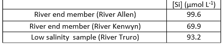
It shows that there was higher concentration of Si in the River Allen, with a value of 99.6 mmol L-1, than the River Kenwyn (69.9 mmol L-1). Therefore by looking at the concentration of the sample from the River Truro (93.2 mmol L-1) it would seem that the River Allen had the greatest input of water, since its value was the closest to that of the Truro’s. If we were to use a sample of 0 salinity for the river end member in our discussion, the river Allen would be the river we would use.

Looking at the mixing diagrams, the estuary behaviour seemed to be inconclusive for each nutrient. This is due to there were not enough water samples collected in the upper end of the estuary. This was down to human error when deciding the location of sampling, and how many samples to take. Furthermore, the data was limited to a range of 29-35 salinity, since the upper estuary was too shallow for sampling with R.V. Bill Conway. This could also be a factor that led to the inconclusiveness of the diagrams.

However, it could also be argued that Figure 12b and Figure 13b could be interpreted as they both show conservative behaviour for silicon and nitrate. These data points seemed as if they were following the TDL. Conservative behaviour shown suggests that the change in nutrient concentrations was down to mixing within the estuary. Our depth profiles for the Fal estuary support this statement since they show that in the lower part of the estuary (station 51-53; see Figures 1-3); temperature, and salinity did not change much with depth. This implies a well-mixed water column. Additionally, conservative behaviour of nutrients indicates that there were no removal or addition of the nutrient by solution reactions or additional sources; hence the concentration of nutrients depends solely on the amount of mixing within the estuary.

Furthermore, Figure 14b suggests that the phosphate was non-conservative in its behaviour, as there was a great removal shown in the lower part of the estuary/offshore. Non-conservative behaviour suggests that differences in concentration of a nutrient, in this case phosphate, was due to active chemical processes occurring in the estuary. However due to the limitation of the mixing diagrams, it was not possible to evaluate what processes had taken place. Smith & Longmore (1980) suggested that the removal of phosphate in estuaries could be due to removal to the sediments. Moreover, as phosphate is limited in estuaries (Nedwell et al, 2002), a clearer picture of nutrient behaviour was shown in Figure 14b.

However, non-linear relationship with phosphate may not non-conservative behaviour. It could be due to additional sources which were exterior to the water column or it may even be due to temporal variability in end member concentrations. This might be true for this particular investigation as the sampling vessel experienced technical difficulty after station 54 and so there was a 2 hour delay before taking the next sample at station 55.

Physical structure and Richardson number of water columns

The overall salinity in the water column decreased as stations moved from lower to upper estuary due to freshwater input; the overall temperature increased due to shallower depth. However a thermocline and halocline were found at station 57 (upper estuary). The range of salinity throughout the estuary was from 29 to 35. This shows the narrow scale of salinities measured; and implies the freshwater inputs had little effect on the results due to location selection for sampling and the depth of keel on the boat.

The overall current velocity in water column increased from lower to upper estuary, however from station 54 to 56 a noticeable difference in velocity between upper and lower water column was detected. This could be due to samplings against tidal movement, leading to stronger current velocity detected on the surface (High tide: 8:40am, Low tide: 2:55pm UTC). This phenomenon was not observed at station 51 and 52 due to they were close to offshore, and was not observed at station 57 due to the depth was too shallow to allow any conclusion to be made.

However, the Richardson numbers calculated for stations 51-54, and 57 contradict the water column structures measured at respective stations by CTD.  No stratification was seen for stations 51-54 as claimed by the peaks shown on Figures 28-31, and stratification was not detected by Richardson number for station 57 (however thermocline and halocline were shown on the depth profile for station 57 (Figure 7)). Since the Richardson numbers were calculated from ADCP data, gaps were shown on ADCP data due to sampling error (see Figures 22-25, and 28), and Figure 28 shows station 57 had mixed velocities throughout water column; these factors might had caused the inconclusive results.

Turbidity, backscatter and plankton communities in water columns

Figure 11 shows that station 51 had the greatest transmission hence had the lowest turbidity; and station 57 had the lowest transmission/highest turbidity throughout their respective water columns. This gives support for the Secchi disc results shown in Table 1; as the light attenuation coefficients increased steadily from station 51 to 54, then a large increase occurred between 54 and 55, and a steady increase from 55 to 57. Thus provides evidence that turbidity was positively correlated with the light attenuation coefficient in the water column.

The rapid increase in light attenuation between station 54 and 55 could be the result of the decrease in cloud cover (by 3/8) between stations, leading to larger amount of light penetrated into the water column at station 55. Such information can be linked to higher amount of phytoplankton were collected in the upper estuary as stations were moved from 54 to 56 (note that no phytoplankton samples were collected at station 55 due to limited amount of sampling bottles). However this alone does not explain why station 56 had the highest amount of phytoplankton detected in surface water, as station 57 had the highest light attenuation coefficient (i.e. highest turbidity) throughout the water column.

The backscatter on the surface water did not vary much along the Fal Estuary, which did not correlate to the increasing number of phytoplankton detected from lower to upper estuary. However backscatter is also a reflection of suspended particles in water column. The bottom backscatter increased steadily from station 54-57. This was caused by changes in depth across stations, and since the effect of tidal movement started to appear on the current velocities in water column due to shallower depth (difference in current velocities between upper and lower water columns as mentioned); friction between upper and bottom water column occurred at stations 54-57. Friction therefore caused higher levels of suspended particles to appear lower in the water column at stations 54-57.

Moreover, although station 57 showed mixed velocities in water column due to shallow depth, the backscatter on the bottom was higher than the surface. This could be due to the overall high turbidity in water column with the factor that station 57 was positioned at a mudflat, caused more particulate matter to re-suspend at the bottom.

The overall backscatter throughout water column increased from lower to upper estuary. This correlates with the transmission and Secchi disc data in which the overall turbidity and light coefficient in water column were also increased upstream. Therefore turbidity, light coefficient and backscatter in the Fal Estuary were in fact affected by certain common factors.

Control of primary production and dissolved oxygen in the Fal Estuary

The phytoplankton community was found to be containing similar amount of phytoplankton species along the Fal Estuary. However the amount of phytoplankton detected in surface water increased as stations moved upstream. This could be due to increasing amount of nutrients (silicon, nitrate and phosphate) were found in water column upstream. However, the mixing diagrams (Figures 12-14) do not show greater removal of nutrients upstream; therefore the measured nutrients concentrations do not correlate with the primary production along the Fal Estuary. This could be due to field (i.e. nutrients) run off in the upper estuary, possibly overriding or balancing the removal of nutrients by primary production in this survey.

The dissolved O2 concentrations measured in the lower water column were positively correlated with the number of phytoplankton collected along the Fal estuary. This shows that primary production controls the dissolved O2 concentrations at lower depths. Although a similar pattern was observed for the dissolved O2 concentration in the upper water column, station 55 had a higher dissolved O2 concentration than station 56, while station 56 had a higher number of phytoplankton detected. This could imply certain species of phytoplankton are more efficient at O2 evolution.

The zooplankton community was found to be more diverse on the surface of lower and middle estuary than the upper estuary, which differed to the pattern observed in the phytoplankton community. The amount of zooplankton decreased dramatically from lower to middle estuary, no recovery of numbers was shown in the upper estuary; while the amount of phytoplankton increased gradually from lower to upper estuary. This was due to the grazing of phytoplankton by zooplankton. As there was a zooplankton maxima in the lower estuary, the phytoplankton biomass was limited by zooplankton in the lower estuary.

Flushing & Residence time

Flushing time describes how long it would take to fully replace the freshwater within the estuary with “new” freshwater from riverine inputs. In the Fal during a Spring tide, this was calculated to be 56.5 hours. The residence time describes how long it takes for every particle within the estuary to leave, and is much longer at 160.6 days.

Both of these are important methods for analysing the impact of pollutants on an estuary – by either calculating how much pollution you can allow to enter without it building up or modelling how a pollution event will affect the estuary. The residence time calculated is very high, which suggests any pollutants entering the estuary would stay there for a long period of time and could therefore accumulate and cause problems.

They can also be useful in determining why plankton communities are established in certain areas. The concentration of phytoplankton was found to significantly increase further up the estuary which could be partially due to a long residence time in this area allowing them to linger instead of being washed away. Due to the strong tidal nature of the Carrick Roads basin reducing the overall residence time, it is likely to be even higher in this less active part of the estuary.

Due to the limited number of stations and locations sampled in the estuary, the average depth calculated could be inaccurate. Because of the large size of the estuary, an inaccuracy of just 1m in depth would result in the estuary volume calculation being out by about 24.5km3.

The tidal prism method used to calculate the flushing time relies on several assumptions. It assumes that the salt water entering the estuary is completely mixed with the fresh water at high tide, and that the combined volume of sea and river water that entered the estuary during the tidal cycle leaves during the falling tide. In reality, not all of this water will leave the estuary and some of it will return during the following tidal cycles. This means that the flushing time calculated is likely to be a slight underestimate of the actual flushing time (Ketchum, 1951). While no estuary will follow these assumptions precisely, they are generally accurate enough to give a useful estimation.

It is also difficult to calculate a single flushing or residence value for the Fal estuary as the upper and lower estuary have such different properties – with the deep tidal basin at Carrick roads (comprising around 80% of the estuary water volume) contrasting sharply with the shallow, narrow, meandering channels further up the estuary.

References

Ketchum, B. H., Rawn, A. M. (1951). The flushing of tidal estuaries.  Sewage and Industrial Wastes, 23(2) pp. 198 – 209

Nedwell, D. B., Dong, L. F., Sage, A., and Underwood G.J.C. (2002) Variations of the Nutrients Loads to the Mainland U.K. Estuaries: Correlation with Catchment Areas, Urbanization ad Coastal Eutrophication. Estuarine, Coastal and Shelf Science. 54(6), 951-970

Simpson, J. H., Williams, E., Brasseur, L. H. and Brubaker, J. M. (2005) The impact of tidal straining on the cycle of turbulence in a partially stratified estuary. Continental shelf research. 25. 51-64

Simpson, J. H., Brown, J., Matthews, J., Allen, G. (1990). Tidal straining, density currents, and stirring in the control of estuarine stratification. Estuaries, 13(2), 125 - 132 pp.

Smith, J. and Longmore, A. (1980). Behaviour of phosphate in estuarine water. Nature Publishing Group

Image 2 | Deployment of the CTD rosette sampler.

Image 1 | Map of the Carrick Roads section of the Fal Estuary and the river Fal. Includes markers for locations of sample points.

Disclaimer- the views shown here are solely of group 10 and do not necessarily reflect the views or opinions of the university of Southampton.

Abstract Introduction Methods Results Discussion

Abstract Introduction Methods Results Discussion

Abstract Introduction Methods Results Discussion

Habitat Mapping Poster Abstract Introduction Methods Results Discussion