


A time series was carried out off the coast of Falmouth over an 8 hour period. Using a CTD, ADCP and chemical analysis, the physiological and organic properties of the water column were studied. A thermocline was a clear feature of the water column, and a high Richardson number around such a thermocline further proved the water column was heavily stratified. Nutrients were found in greater abundance around the thermocline, and coupled with that, a higher level of fluorescence, and thus phytoplankton. To act upon the large levels of phytoplankton, a wide diversity of Zooplankton orders were found below the thermocline.
During the spring, due to solar heating and weak current the surface layers of the
sea will become stratified in offshore Falmouth (Larsonneur et al., 1982). This layer
of hotter water will be nutrient rich due to winter upwelling and will normally lead
to blooms of diatoms (Menesguen and Hoch, 1997). These blooms in spring will deplete
nutrients in the surface layer and die off due to lack of available nutrients (Menesguen
and Hoch, 1997). Therefore by mid-
The aim of this study was to assess the effects, indirect or direct if any, of vertical mixing on the temporal variability of the plankton communities and their structure by looking at the behaviour of nutrients throughout the water column. As well as this we wanted to look at the changes mentioned throughout the day and show their variability within the tidal cycle.
Irigoien et al. (2004) demonstrated that the micro-
Rosette Sampler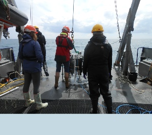
We used a rosette sampler equipped with 8 Niskin bottles and a CTD, which recorded temperature, salinity and fluorescence (to measure chlorophyll concentration). It was lowered to roughly 5m above the sea floor at each station and the CTD profile of the descent was used to determine where to collect samples during the ascent. Three samples were taken using the Niskin bottles at each location with one near the sea floor, one during the chlorophyll maximum and one near the surface – the collection of which was triggered remotely from the boat.
Plankton net
A plankton net (mesh size 200µm, diameter 0.5m) was deployed at each station twice (three times at the first station) at different depths. The depths were determined based on areas of interest identified on the CTD profile (at the chlorophyll maximum and another below where zooplankton are likely to conjugate).
Laboratory – Callista
Samples taken from the plankton nets and the Niskin bottles were processed and preserved
in the on-
Laboratory – Falmouth
In the laboratory, phytoplankton and zooplankton samples were counted and identified using light and stereo microscopes respectively. These values were then converted to give an average concentration of plankton at each recorded depth in every station.
The water samples were then analysed to give us readings for O2, phosphate, nitrate, silicon and chlorophyll.
Figures 1-
Temperature
Throughout the tidal cycle from 08:30-
At 08:30 the thermocline initially ranges from 15-
Initially starting at ~10m the thermocline widened at 11:30 (Figure 5) to a depth
of ~25m; however this has disappeared by low tide at 12:30 (Figure 6); where the
thermocline descended to ~20-
As the tide ebbed, a descent of the thermocline was observed, with a subsequent ascent
initialising at 14:30 following low tide at 13:30 (Figure 3). The descent of the
thermocline coincided with improved mixing of the water column below the thermocline;
the temperature remaining at a constant 13oC from 25-
Salinity
Whilst no halocline is present (Figure 10), a clear temporary decrease in salinity can be observed throughout the time series for the duration of the thermocline (Figure 1,2,4,5,6,7,8,9). Two areas of much higher salinity are visible at 09:30 where salinity rises to 36.2 from 35.0, and at 15:30 where a smaller increase from 35.0 to 35.4 is observed. The former spike in salinity coincides with that observed in temperature and density, whilst the latter is only clearly visible in salinity. However it must be noted that the beginnings of a similar small area of great increase are visible in both density and temperature (Figure 3,11).
Density
The pycnocline maintained a similar structure to the thermocline throughout the tidal
cycle (Figure 11). Water density ranged from 1025-
Slight stratification below the pycnocline is visible. ~25-
Fluorescence
Fluorescence has been used as a proxy for chlorophyll and thereby phytoplankton growth.
Highest fluorescence levels can be observed just below the thermocline at the chlorophyll maximum (Figure 12).
From the surface to the chlorophyll maximum little fluorescence occurred throughout
the time series, with the lowest levels (-
At 13:30, low tide, fluorescence reduced at depth to 0.08, occurring only at the
chlorophyll maximum, for the width of the thermocline (Figure 6). Prior to this a
second peak in fluorescence (0.16mg/m3) was visible at ~40m (all multiline plots
from 08:30-
Figures 13-
Chlorophyll
Chlorophyll follows the same structure as fluorescence, (Figure 13) with low levels
in surface waters, increasing from ~0.6mg/L to 1.5-
Between 08:30 to 13:30, a second peak in chlorophyll can be identified at ~45m where
chlorophyll rises to a maximum of 3.2mg/l at 15:30 before returning to its steady
level of 1.0-
O2 (%)
Few changes in dissolved oxygen occur during the time series (Figure 14). At the
surface dissolved oxygen ranged from 103-
Silicate
For the majority of the time series, dissolved silica remained between 0-
Nitrogen
From the surface to ~25m nitrate concentrations remain relatively constant between
0-
At low tide (13:30 UTC) nitrate concentrations were a constant 1.6 μmol/L between
0-
Phosphate
Across the tidal cycle, phosphate is constantly changing (Figure 17). In general
at the surface, concentrations vary between 0-
At the thermocline a gradual increase in concentration can be observed until low tide, starting at 0.05 μmol/L at 08:30 UTC, reaching 0.25 μmol/L by 10:30, peaking at 11:30 (0.45 μmol/L) before dropping at low tide (13:30) to 0.09 μmol/L, where the decrease continues to 14:30 (0.15 μmol/L) before increasing to a final concentration of 0.38 μ mol/L.
There is no visible pattern at depth. Phosphate concentrations began at -
Figures 18-
Water Column Structure
Due to lack of data for 08:30-
From the calculated Richardson numbers, it can be seen that the majority of the water column remains well mixed (Figures 18, 19, 20, 21). From low tide at 13:30 to 16:30 UTC, a layer of stratification remains present at 30m. This is most prominent at 13:30 and 16:30, reducing to ~10 from ~30 at 13:30 and increasing to ~60 at 16:30.
A second layer of stratification (Ri of ~40) is present at 14:30 at a depth of 45m.
This is visible at all other times, however is far less prominent, with Richardson
numbers of 2-
A final layer of stratification is visible at ~55m. Whilst this remains throughout the time series, the depth varies from ~58m at 13:30 to a double layer at 53 and 58m at 14:30. The stratification layer remains at 53m at 15:30 before dropping to 55m at 16:30.
Figures 22-
Phytoplankton
The dominant genera of phytoplankton at the offshore station were Chaetoceros, Guinardia and Leptocylindrus, with Leptocylindrus being present in notably larger quantities than the other genera at all but the first sample at 13:30 UTC (Figure 22). At 15:30 UTC (Figure 23) there was a more consistent spread of plankton between the different genera while all other times show the 3 dominant genera outnumbering the others.
When the data is broken up by depth, very little plankton were present near the surface at the beginning (13:30 UTC) and end (16:30 UTC) of the afternoon time series (Figures 24, 25)) despite these samples having a much higher number of total plankton than the two middle samples (at 14:30 and 15:30 UTC). The two middle samples had a more consistent spread of plankton numbers across all 3 depths. The most dominant genus (Leptocylindrus) generally preferred lower depths of between 25 and 55m and was only found in substantial numbers on the surface at the 15:30 UTC sample.
Figures 28-
Zooplankton
Figure 28 shows the numbers of different zooplankton orders at station 41 at depths
0-
Following station 41, only two plankton nets were sampled at the latter stations,
one near the surface and one under a recorded high fluorescence (recorded on CTD
data). Figure 29 shows the plankton nets at station 42. Similar to station 1, the
deeper depths had greater diversity of zooplankton orders, with 6 at depths 15-
A much similar trend to the previous stations can be seen at station 43 (Figure 30).
Cladocera dominates the water column at a depths of 0-
Such a trend continues at the last station sampled, station 44 (Figure 31), However,
was can be noted is that Cladocera are no longer the most prevalent order present
close to surface. In the plankton net 0-
Figures 32-
ADCP
The change in tides can clearly be seen in the ADCP velocity magnitude (Figure 32) and ship track profile (Figure 33). The turn of the tide occurred at 14:30 UTC, following low tide at 13:30 UTC halfway through the afternoon time series. Note no data is currently available for the morning time series due to it being completed by another group.
Before and after the change in tidal state, areas of higher velocity are present.
At the change in tide, velocity drops completely, before reversing direction and
increasing back to original levels of 0.3-
ADCP can also be used to observe zooplankton and other objects in the water column, such as shoals of fish. Throughout the transect, a persistent layer of zooplankton was present at ~35m, just below the thermocline (Figure 34, although this did decline slightly when the tide turned at 14:30 UTC.
Approximately at 15:30-
From the temperature contour it can be seen that the depth of the thermocline increases as the tide goes out. The tide height reaches a minimum of 0.8m at 12:25 UTC. At 08:30 UTC the bottom of the thermocline sits at approximately 21m and this depth decreases as the tide moves out, reaching a depth of approximately 30m at 13:30 UTC. The phytoplankton move with the thermocline so the increase in the depth of the thermocline causes the depth of the chlorophyll maxima to increase.
There is no halocline present in the data, which shows that the water column is well mixed. The spikes in slight increases in salinity seen around the thermocline are due to the CTD measuring salinity from conductivity, causing an error in the measurement until the CTD corrects itself. This is due to lag from the temperature measurements, which causes CTD to constantly correct itself as the CTD descends past a strong thermocline.
After 13:30 UTC the tide begins to flood, from the Richardson numbers it can be deduced
that the water column becomes more stratified as the tide comes in. The temperature
of the surface water increases due to solar energy. Between 15-
A small pocket of high salinity, low temperature water can be seen at 09:00-
Fluorescence maxima (indicative of chlorophyll maximum) can be seen below the thermocline
throughout the time series. Phytoplankton typically dwell just above the thermocline
area due to an increase in available nutrient. Excluding some cases of silicate,
which are higher near the surface, nutrient levels typically increase below the thermocline.
This is caused by blooms in the upper water column in earlier months, which deplete
the nutrient levels in the upper water column, and thus-
Needing sunlight to photosynthesise, phytoplankton will remain at a depth at which
sufficient light and nutrients are available. Phytoplankton thus thrive just above
the thermocline, where there is more nutrients than at the surface waters, and enough
sunlight to photosynthesise. These nutrients are supplied by turbulence around the
thermocline, and thus providing bottom layer nutrients for production (Sharples et
al, 2001). Due to its unique physiological features, there are a vast amount of phytoplankton
above the thermocline, so much so that they contribute 20-
If the water is deeper, it is seen that there is a greater diversity of zooplankton.
This can be seen in all four figures (Figures 27-
In the upper water column Cladocera are a very prominent genus. It is well documented that where there is a large amount of phytoplankton, there is typically a large amount of Cladocera, with Cladocera being one of the most common zooplankton to be encountered (Frey & David, 1987). It is likely competition which drives the Cladocera to the surface water, surviving against predation by their sheer numbers (Stibor & Herwig, 1992).
The ADCP shows a tidal change at approximately 14:30 UTC, This could account for lower nutrient levels in the water column past 14:30 UTC. The nutrient richer estuarine waters begin moving inland, rather than moving out with the tide to supply the coastal waters with nutrients, and in its stead is the nutrient poor waters from further away from shore. Because of this, the nutrient levels decrease significantly.
References
Frey, & David, G. (1987).The taxonomy and biogeography of the Cladocera. Cladocera.
Springer Netherlands, 5 -
Irigoien, X., Huisman, J., & Harris, R. P. (2004). Global biodiversity patterns of marine phytoplankton and zooplankton. Nature, 429(6994), 863 – 867 pp.
Larsonneur, C., Bouysse, P., & Auffret, J. P. (1982). The superficial sediments of the English Channel and its western approaches. Sedimentology, 29(6), 851 – 864 pp.
Menesguen, A., & Hoch, T. (1997). Modelling the biogeochemical cycles of elements limiting primary production in the English Channel. I. Role of thermohaline stratification. Marine Ecology Progress Series, 146(1), 173 – 188 pp.
Paulson, C. A., Simpson, J. J., (1977) Irradiance Measurements in the Upper Ocean. J. Phys. Oceanogr., 7, 952 – 956 pp.
Pingree, R. D., et al. (1982) Vertical distribution of plankton in the Skagerrak
in relation to doming of the seasonal thermocline. Continental Shelf Research 1(2),
209 -
Revelante, N. and Gilmartin, M. (1973) Some observations on the chlorophyll maximum and primary production in the Eastern North Pacific. Internationale Revue der gesamten Hydrobiologie und Hydrographie. 58(6), 819 – 834 pp.
Robinson, G. A., & Hunt, H. G. (1986). Continuous plankton records: annual fluctuations of the plankton in the western English Channel, 1958–83. Journal of the Marine Biological Association of the United Kingdom, 66(04), 791 – 802 pp.
Sharples, J., Mark Moore, C., Rippeth, T. P., Holligan, P. M., Hydes, D. J., Fisher, N. R. and Simpson, J. H. (2001) Phytoplankton distribution and survival in the thermoline. Limnol. Oceanogr., 46(3), 486 – 496 pp.
Stibor, & Herwig. (1992) Predator induced life-

Meta Data
Date: 28/06/2014
Time: 13.25
Location: 50°05’610”N 004°52’961”W
Low Tide: 12.25 (0.8m)
High Tide: 05.42 (4.8m), 17.56 (5.0m)
Light Wind
8 octants cloud cover (light rain) reducing to 2 octants
(All times in UTC)
Image 1 | CTD rosette pre-
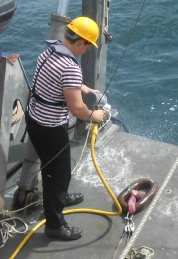
Image 2 | Cleaning of the zooplankton net.
Disclaimer-
 Back to Top