
Callista - Offshore Biological and Chemical Analysis
| Return to Home Page | Grey Bear - Geophysics | Bill Conway - Estuarine Analysis | Ribs - Estuarine Analysis |
|
AIMS:
To investigate whether biological succession of phytoplankton and zooplankton species along a potential physical gradient from the Fal estuary to offshore waters can be observed. Also, to establish an understanding of the water column in offshore waters by looking at various physical parameters.
OBJECTIVES:
Using ADCP readings to determine physical fronts found between different bodies of water, CTD drops can be conducted with a view to building up a detailed knowledge of the vertical profile of the water column. Biological and chemical analysis can be carried out using the samples to determine any succession that is occuring.
METHOD:
An ADCP was used along two separate transects, the first travelling from North (Lat: 050°05.074, Long: 004°57.561) to South (Lat: 050°05.072, Long: 004°57.394) and the second from South (Lat: 050°06.414, Long: 004°54.285) to North (Lat: 050°08.352, Long: 004°56.016). The two transects ran across a suspected offshore front. The ADCP was also used at each station to take a time series while the CTD was deployed overboard. The CTD was deployed at 8 separate stations at depths of up to 40 metres. A transmissometer, fluorometer and rosette were attached to the CTD. The rosette had 5 Niskin bottles attached allowing water from a variety of depths to be collected. A vertical closing zooplankton net was deployed at 6 of the 8 stations and two separate depths at stations 3 and 5. A secchi disc was deployed at each station to provide a valuable indication of light penetration through the water column.
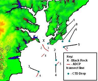
Figure 1 - ADCP transect lines and CTD deployment sites for the Callista boat practical, 13th July 2006
In terms of zooplankton, we were interested to see how they would vary across any frontal feature we could locate, along with their potential food source. To classify and quantify the zooplankton species at each station first a CTD downcast located any chlorophyll maxima. These were the areas we were interested in sampling as we made the assumption that any zooplankton would follow the migration of their food source. The depth at which this fluorescence peak started and finished was then sampled using a vertical trawl using a net filter size of 200 mm, with a messenger weight closing the net at the finish depth. A small sample was then immediately analysed under the onboard microscope and the rest of the water was treated with a small volume of formalin to kill any zooplankton to prevent further grazing. Samples of water from each depth were filtered and stored for nitrate, phosphate and silicate analysis. Oxygen samples were fixed on board ready for later analysis in the laboratory and chlorophyll was filtered and stored in acetone. 100ml of the water samples from the different depths was mixed with Lugols Solution to stain the phytoplankton present.
RESULTS:
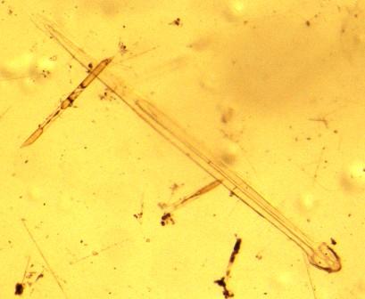
ZOOPLANKTON - There were notable trends in zooplankton abundance and diversity along a gradient running from the mouth of the Fal estuary to an offshore position. Copepods showed high abundance further offshore, stations 2 and 3 had numbers in excess of 3000 (refer to Figure 7) individuals per cubic metre. However, at station 4, which was predicted to be on the offshore side of a front, showed results closely correlated with the inshore readings, around 1700. The copepod abundance at Black Rock (station 1) and nearby stations was around 1500 individuals per cubic metre. An anomaly occurred at station 6 with numbers of individuals over 4000 per cubic metre. Calanoid copepods were found at all stations, while some Cyclopoid copepods were found only at station 7, to the west of the mouth of the estuary. Chaetognaths (Figure 2) showed the opposite relationships to copepods, with the greater numbers being found inshore and low numbers on the offshore side of the predicted front. There were only 50 individuals per cubic metre at station 4 and 500 at the other three offshore stations. The inshore stations recorded numbers of Chaetognaths between 1000-1400 individuals. Cladocerans were only found at stations on the inshore side of the predicted front. Numbers of individuals ranged from 100 per cubic metre at station 1 to 500 per cubic metre at the lower depth of station 6. One site further offshore contained Cladocerans, station 2 had around 600 individuals per cubic metre.
2
 3
3
 4
4
 5
5 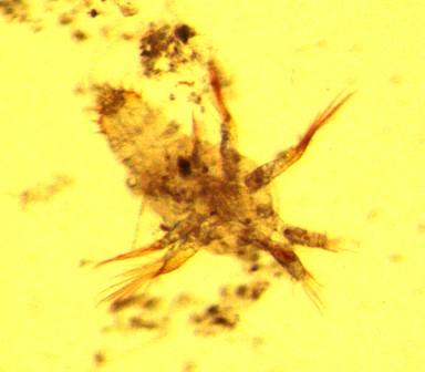 6
6
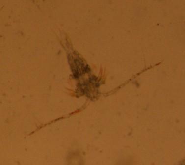
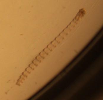
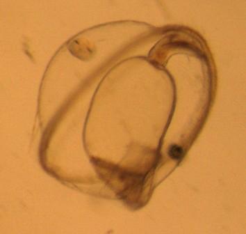
Figure 2 - Chaetognath, Figure 3 - Polychaete, Figure 4 - Trocophore, Figure 5 - Nauplius larvae, Figure 6 - Pelagic Copepod
Diversity also shows a gradient, with diversity increasing closer to the mouth of the estuary. The station furthest from the mouth of the estuary and most likely to be beyond the coastal front has the lowest diversity of zooplankton. Only 5 distinct groups of species were found in the deep trawl at station 3 and only 6 in the shallow trawl. However, the station in the mouth of the estuary showed 10 different groups of species, double the amount found furthest from the estuary.
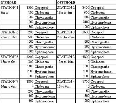
Figure 7 - A table to summarise zooplankton diversity and abundance data collected on Callista, 13th July 2006
NUTRIENTS - ‘Before Front’ where waters are well mixed and stations are closer to the shoreline, Stations 1, 6, 7 recorded data for the area. ‘After Front’ where the waters are highly stratified, stations 2, 3 and 4 recorded data from this area of the frontal waters. The data recorded at these stations gives a broad spectrum of chemical, physical and biological activity over a front.
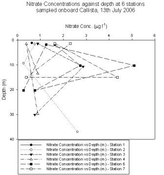
Nitrate - Lower nitrate (Figure 8) concentrations were found at the surface in ‘after front’ stations opposed to ‘before front’ stations. For example, the value of the surface concentration of nitrates of station 2 is 0.75µmol compared to station 7’s concentration of 1.6224µmol (0.8724µmol difference). All nitrates values increase at ‘mid depth’ values with station 2 being the exception. Large increases were often seen, with a three fold increase at station 7. These mid depths ranged from 10-15metres. Deep water samples show a decrease in nitrate concentration returning to levels seen in surface waters. Again station 2 is the exception which sees a further increase in concentration from the mid depths (0.26-2.61µmol). Nitrate Max- 4.35µmol at 15 metres, station 7. Nitrate Min- 0.26µmol at 9.4 metres, station 2.
Silicate - There was high silicate (Figure 9) utilisation and therefore low concentrations in the ‘after front’ stations in surface waters. This contrasts with the ‘before front’ surface concentrations which had higher silicate values (Station 3- 2.1µmol, Station 6- 2.35µmol) ‘Before front’ stations all show a decrease in Silicate concentrations towards mid depths and then increase to lower depths. ‘After front’ stations show varying fluctuations in mid and lower depths. Station 2 increases in concentration at mid depth and then further to 2.54µmol at 37 metres. Silicate Max- 2.54µmol at 37 metres, station 2. Silicate Min- 2.107µmol at 1.4 and 10.7 metres, station 3.
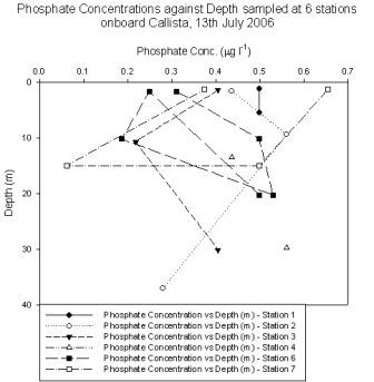
Phosphate - All ‘before front’ mid depths converge a phosphate (Figure 10) concentration very close to 0.5µmol. This value then changes very little when passing to increasing depths to 20.24 metres. ‘After front’ values vary but the general pattern is of a surface value close to 0.43µmol. Mid depth concentrations range from 0.22 to 0.56µmol with 2 of the 3 stations increasing to higher phosphate values at lower depths. Phosphate Max- 0.65µmol at 1.3 metres, station 7. Phosphate Min- 1.25µmol at 1.7 metres, station 6.
8
 9
9
 10
10
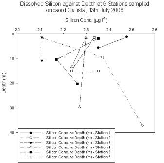
Figures 8 (Nitrate), 9 (Phosphate) and 10 (Silicate) - Graphs to show the relationship between nutrients and depth at the 6 CTD sites, 13th July 2006
Click on image to enlarge
ADCP - 8 transects were surveyed during the Callista boat practical. It was later decided that analysing all this data was unnecessary so only the transects from before, during and after (2, 4 and 5) the major physical front were processed.
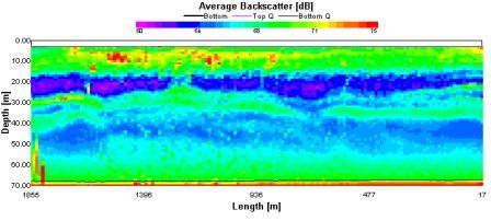
Transect 2 - On reaching station 1 the vessel proceeded at a 6kt speed to allow ADCP transects in which it was planned to observe a front that the group intended to pass, analyzing phytoplankton species on both sides of and in the front itself. The thermosalinograph recorded a distinct rise in temperature at a location of 50°05.245N, 004°57.589W which was unanimously decided by the group to be the front (Figure 12). From analysis of the onboard thermosalinograph it was decided that at a scan count of 1600 the vessel had passed through the front and an ADCP transect was taken at this time to investigate what the group perceived to be the seaward side of the front (Figure 11). The ADCP picked up what appeared to be a plankton bloom at 30m prompting a CTD drop. Samples were taken at the surface, 9.4m and 37m. The 9.4m sample being taken due to an unusually high level of fluorescence recorded on the CTD and 37m for the presumed zooplankton bloom (X:\group12\callista\proc data\CTD\Station2ctd)
The velocity magnitude profile shows a distinct boundary in the horizontal profile at approx. 5500m. On the seaward side the water column was travelling uniformly towards 180°, on the estuarine side of the front the water was travelling uniformly at 230°.
11
 12
12
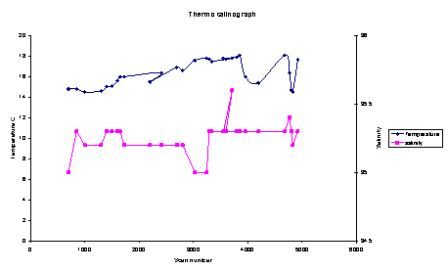
Figure 11 - ADCP backscatter profile of transect 2
Figure 12 - Thermosalinograph profile showing temperature and salinity readings throughout the boat practical
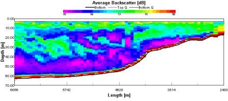
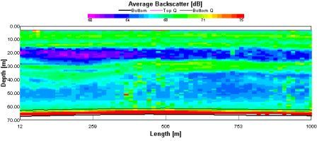
Transect 4 - A front was observed on the thermosalinograph at an approximate location of 50°05.245N, 004°57.589W. It was decided to transect a region beyond the front to investigate the plankton species further out to sea. To accomplish this, the vessel cruised at 6kts running a continuous ADCP transect in search of a plankton bloom. Figure 13 shows what was thought to be a bloom discovered at a position of 50°01.734N, 004°53.074W. The surface layer is presumed to be the euphotic zone due to the strong backscatter recorded. Beneath which is a layer of clear oceanic water at a depth of 20-30m, probably nutrient poor. At a depth of 30-40m there was a considerably large layer of backscatter detected which could have been associated with another zooplankton bloom, which as mentioned previously is a likely sign of phytoplankton. Below this layer there were intermittent areas of backscatter. A CTD profile was taken (X:\group12\callista\proc data\CTD\Station3ctd) and high levels of fluorescence were recorded at 30m and 10.7m. Samples were taken of these two depths and at the surface for further analysis at the laboratory.
13
 14
14
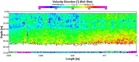
Figure 13 - ADCP backscatter profile of transect 4
Figure 14 - ADCP velocity direction profile of transect 4
Transect 5 - At an approximate position of 50°04.432N, 004°53.931W an abrupt increase in temperature and a decrease in salinity were observed on the thermosalinograph (Figure 12). It was decided to run an ADCP transect in order to ascertain any reasoning behind the temperature anomaly. Figure 15 shows a section of backscatter from the transect recorded. From 0-15m there is strong backscatter which was taken to be the euphotic zone; this was followed by a 5m layer of low backscatter taken to be clear oceanic water below which was the key finding of a strong layer of backscatter at 30m. In view of the groups initial aim of zooplankton identification a CTD deployment was taken with the intention of correlating fluorescence recordings with the backscatter. Results indicated a trend therefore the backscatter was taken to be a zooplankton bloom and samples at 29.7, 13.5 and 1.5m were taken for further analysis in the laboratory.
15
 16
16
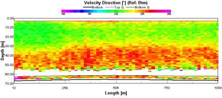
Figure 15 - ADCP backscatter profile of transect 5
Figure 16 - ADCP velocity direction profile of transect 5
PHYTOPLANKTON - There was a relatively high diversity found in these samples, with twenty two species recorded across the samples with diatoms, ciliates, dinoflagellates and flagellates all represented. Even though there was an overall biodiversity, at single stations diversity could be low, for example at station 2 (37m), only three species were found. Numbers varied greatly between sites and depths. At the majority of sites the numbers were highest in surface waters whereas at others, such as station 4, the surface abundance was the lowest of all three depths. The highest recorded overall was a sample taken from station 7 at a depth of 1.3m with a frequency of 745 cells per 100ml. The lowest of any samples was from sample 2 at 37m with only 70 cells recorded. Refer to Figure 17 below.
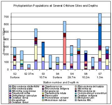
Figure 17 - Bar chart of phytoplankton species diversity from the Callista boat practical, 13th July 2006
DISCUSSION:
ZOOPLANKTON - The reason for the high levels of copepod abundance at station 6 may be due to the close proximity of the station to the predicted front. It is possible that copepods thrive in the conditions at a front and their dynamic ability allows them to capitalise on the high levels of phytoplankton that would be expected in a frontal zone. The high numbers of zooplankton also correlate closely with data recorded from the ADCP which picked up high levels of backscatter towards the end of the transect, finishing nearby the position of station 6.
The increasing offshore diversity gradient is unexpected to a certain extent. More stabilised conditions were expected offshore which should lead to a collection of equilibrium ‘k’ selected species and higher diversity. In fact, the diversity appears to increase closer to the shore. When analysed alongside the data collected from the ADCP and vertical profiles from the CTD, the diversity gradient complies with the physical environment. Although stations 2-4 were expected to be beyond a front, analysis has shown that there was little or no stratification and no truly stable conditions. This suggests that the low diversity offshore is due to the changeable physical environment, and consequently the presence of more pioneering ‘r’ selected species, or simply those species better adapted to cope with the unstable physical environment.
NUTRIENTS - Silicate concentration is low in the surface waters in the ‘after front’ samples, indicating high levels of diatom production in the more stable waters. This region of high productivity reducing silicate concentrations correlates well with nitrate concentrations which are also at a decreased level in the surface waters after the front. This reduction in nitrate and silicate concentrations is likely to be due to the gradual formation of stratified waters after the frontal region allowing more light to penetrate further into the water column. This allows for an increase in primary production. In a summer bloom, diatoms are the first to increase in biomass size on an exponential scale due to the reduced need for high light levels and this is represented in stations 3 and 4.
While diatoms are dominant surface waters after the front, flagellates are the most common phytoplankton in mid depth waters. Flagellate species require lower nitrate levels to grow and an increase is seen from the surface waters where the nutrient demanding diatoms are found. This change in phytoplankton type is represented by the increase in silicate as flagellates are less reliant on it for their cell structure. Generally speaking, all nutrients increase at the lowest depths. This is because of the recycling that occurs through the microbial loop and other recycling processes allowing nutrients to be re-used. ‘Before front’ levels of nutrients appear to show diatom levels to be highest at mid water depths. This position in the water column is utilised as the chlorophyll maximum will be found here where the optimum nutrient availability and light attenuation allow for prime photosynthesis rates.
Phosphate concentrations are seen in lower concentrations than nitrates and silicates as the Redfield Ratio governs the quantities in which it’ll be found in open ocean waters (N:P~16:1). This is why values of 0.4-0.5µmol are seen compared to nitrate concentrations of up to 4-5µmol. The plots of phosphate concentrations appear to have no or little relevance with reference to depth and position. If put on a larger valued axis for phosphate concentration, there may be more of a pattern in the data. As phosphate values will be higher in more estuarine waters, a transect graph along a salinity gradient with the plots seen in the phosphate graph (the mouth end of the estuary), a more coherent pattern is likely to be seen.
ADCP
Transect 2 - Productivity in this region was expected to be high since fronts are often observed to be regions of high chlorophyll biomass (Pingree et al 1975). The clear layer of oceanic water at 10-20m supports the theory of fronts separating the low nutrient, stratified surface water from higher nutrient mixed water. The large patterns of backscatter recorded at the 20-40m level could have been a result of phytoplankton consuming the nutrients and in turn being grazed on by zooplankton, which showed up on the ADCP. Because the water was more stratified and less turbulent the predominant phytoplankton species could be expected to have been dinoflagellates or flagellates. This can be related to the summer subsurface bloom seen in the thermocline at 25m in May to September which is driven by regenerated NH4; dinoflagellates and flagellates replace diatoms. Plant mass falls to the bottom of the mixed layer and the seafloor because diatoms develop quicker than herbivore biomass.
Water driven along the English Channel coast by westerly and west south-westerly wind fields which has previously had a more northerly origin or influence. However, southerly winds tend to collect water in the entrance to the channel that has originated from the Armorican Shelf region. This interpretation has considerable significance for the concept of plankton indicator species derived from north western and south western sources and could have been considered in further analysis had a more significant investigation of the region taken place. Thus, from the limited amount of data and time available it was not possible to determine long term trends but it was possible to observe how productivity varied over a front.
Transect 4 - The higher backscatter recorded below the bloom could be interpreted as a sign of partially mixed or mixed water, certainly not as clear as the layer recorded below the euphotic zone. This is possibly due a sub surface current that was recorded on the ADCP (Figure 14). The backscatter was presumably being caused by bubbles and suspended particulate matter. Given that fronts are two bodies of water the ADCP profile did not show a stratified water column nor did it portray a totally mixed water column. It can be summarized therefore that even though the profile was taken at a location thought to be beyond the front, the front and its characteristics extended further than at first anticipated. Given more time a higher sampling resolution could be used to show the true extent of the front.
Transect 5 - The velocity magnitude and direction, also measured by the ADCP showed a shear in flow seen in Figure 16. At approx 0-30m the flow which was predominantly 210° was sheared by a bottom current flowing 250°. Shear flow causes turbulence at the boundary layer which here is observed at 30m. The interacting of the two flows at the boundary causes friction and replenishment of nutrients in the upper layers of the water column occurs. Phytoplankton blooms exist in nutrient rich waters although this cannot be confirmed by the ADCP as the resolution is too low. This is a possible reason for the observed zooplankton bloom in Figure 15 as it is most likely that where zooplankton blooms occur phytoplankton blooms are also present. Due to the turbulence of the water column it was predicted that the predominant species of phytoplankton would be diatoms as they thrive in these conditions due to their robust nature.
PHYTOPLANKTON - There were more cells recorded from the sites within the estuary side of the front just slightly offshore. This suggests that the estuary waters are more favourable for phytoplankton to grow than offshore in the main stretch of the English Channel. Due to the warming effect of the Gulf Stream, the English Channel only stratifies properly at the peak of a hot summer. Therefore, later in the year the channel may settle and populations will increase.